Team:Aix-Marseille/Model
Our model aims to show the impact of an effective TB diagnostics test and some other variables on a given population. Our main inspiration was the model created by Abu-Raddad et al. The World Health Organization (WHO) participated in the elaboration of this model using known data.
Our simulations show that an increase in the diagnosis efficiency could help to stop the disease spreading. Moreover an increase of diagnosis efficiency of the smear positive state, the most infectious one, has the biggest impact on the disease propagation. If you want to test it, you'll find the model here.
The modeling tool
To write our model, we used Tellurium notebook. The tool provides a graphical interface to write code and convert it into mutliple standard formats. Tellurium uses Python, R and Markdown. It also implements antimony, a human readable analog of systems biology markup language (SBML). This Made code writing a bit more easier and more efficient. To run simulations, Tellurium uses libRoadRunner, a powerful simulation engine made for systems and synthetic biology.
Introduction
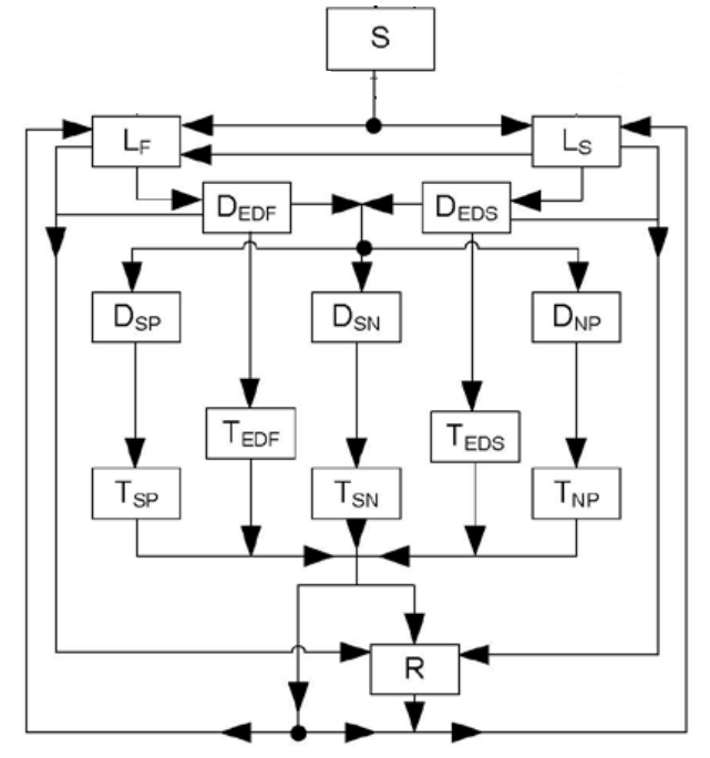
The model is based on multiple works on Tuberculosis epidemiology, making it quite robust. There are multiple epidemiological states in the model:
- Susceptible
- Latent infection
- Early disease
- Treated early disease
- Disease
- Treated disease
- Recovered
The model has two main branches: one for the susceptible population and an other for the vaccinated population. We decided to focus on the susceptible branch to make the model easier to understand. The population is divided into distinct age groups. Thus, the parameter wasn't taken into account.
There are 14 populations in the chosen branch:
- Susceptible (S)
- Latent infection slow progressor (LS)
- Latent infection fast progressor (LF)
- Early disease slow (DES)
- Early disease fast (DEF)
- Treated early disease slow (TES)
- Treated early disease fast (TEF)
- Disease smear positive (DSP)
- Disease smear negative (DSN)
- Disease non-pulmonary (DNP)
- Treated disease smear positive (TSP)
- Treated disease smear negative (TSN)
- Treated disease non-pulmonary (TNP)
- Recovered (R)
Model descrption
The susceptible (S) population represents the born people that can be infected at a rate of infection lambda. Newly infected people can be assigned to two latent states, slow (LS) or fast (LF), determined by the proportion pF. These two populations represent the proportion of infected people that stay in latent infection for a while whereas the other part goes to clinical disease faster due to environment factors. LS population can be re-exposed to the infection and proceed to LF infection. As they were already exposed to the infection, the penetration is reduced by the susceptiblity to reinfection named q. Finally, the rates of proceeding from latent state to early disease states are denoted wls and wlf for the latent slow and the latent fast population respectively.
People in the early disease state can leave this state by four ways, tuberculosis-related mortality, denoted theta, spontaneous recovery, named nu, progression to TB disease, denoted PIE or detection and treatement of early disease X*z, where X is the diagnosis/treatment rate and z the diagnosis efficiency.
Individuals who are diagnosed and treated in the early disease state proceed to treated early disease state. There are still two form, the slow and the fast states. Each individual can leave this state by either, tuberculosis-related mortality, theta, spontaneous recovery, nu, successful completion of treatment phi or re-infection lambda(1-q).
The TB disease state is split into three clinically and epidemiological relevant forms, smear-positive pulmonary (DSP), smear negative pulmonary (DSN) and non pulmonary (DNP). The pulmonary forms of the disease are the only to be considered infectious, having also varying infectious degrees. TB disease individuals can leave this state by either tuberculosis-related mortality, theta, spontaneous recovery, nu or detection and treatment of early disease, X*z. All these movements are modeled as rates and are specific to each form of the disease.
As there are three disease forms, there are three treated disease states each one corresponding to a TB disease state, treated smear-positive pulmonary (TSP), treated smear negative pulmonary (TSN) and treated non pulmonary (TNP). Treated individuals can leave this state by either tuberculosis-related mortality, theta, spontaneous recovery, nu, successful completion of treatment phi or re-infection lambda(1-q). All these movements are form-specific are modeled a form-specific rates.
All individuals who proceed to recovery state (R) can leave this state by natural mortality or through re-infection lambda(1-q).
The force of infection lambda is a function of time and depends on the respiratory contact rate within a population (CR), the probability of transmission per respiratory contact (U), relative infectivity of TB diseased persons with respect to the infectiousness of smear-positive pulmonary TB diseased persons (h), and TB disease and early disease prevalence.
Diagnostics impact
The case detection rate is modeled as equivalent to the treatment rate, assuming that a diseased indivdual positively diagnose will undergo treatment. Each disease state has its own case detection rate (X). This way, we have:
- the case detection/treatment rate for early disease slow (Xes)
- the case detection/treatment rate for early disease fast (Xef)
- the case detection/treatment rate for disease smear positive (Xsp)
- the case detection/treatment rate for disease smear negative (Xsn)
- the case detection/treatment rate for disease non pulmonary (Xnp)
The diagnosis efficiency (z) is modeled to increase the case detection rate. We assume that the treatment duration (phi) does not change in the simulation and is set to 6 months.
Model parameters
The following table encloses the model's parameters. To show the impact TB on the population, we've set the natural mortality rate (mu) to 0.014 and the birth rate (pie) to 20. This way, the population is stable without TB cases (plot).
| Parameter definition | Symbol in the model | Parameter value |
|---|---|---|
| Population model | ||
| Natural mortality rate | mu | 0.014 (per year) equivalent to 70 years life span |
| Birth rate | pie | 20 |
| Disease progression model | ||
| Mortality rate for Smear positive pulmonary TB per year (4 year life expectancy) | theta_sp | 0.25 |
| Mortality rate for Smear negative pulmonary TB per year (10 year life expectancy) | theta_sn | 0.10 |
| Mortality rate for non pulmonary TB per year | theta_np | 0.10 |
| Fraction of fast developpers | pF | 0.9 |
| Resistance to re-infection | q | 0.650 |
| Progression from latent slow to early disease | wls | 0.00075 |
| Progression from fast slow to early disease | wlf | 1.64 |
| Spontaneous recovery | nu | 0.01 |
| Progression to TB disease | PIE | 2.0 (6 month in average = 1/ED) |
| Probability of fraction or relative number of smear positive | pSP | 0.6 |
| Probability of fraction or relative number of smear negative | pSN | 0.2 |
| Contact rate (number of contact per time) | CR | 0.05 |
| Probability of infection per respiratory contact | U | 0.20 |
| Early TB disease duration | ED | 0.5 |
| Relative infectivity of smear positive | hSP | 1 |
| Relative infectivity of smear negative | hSN | 25 |
| Relative infectivity of non pulmonary | hNP | 0 |
| Rate of infection | lambda | CR * U * (hSP * DSP + hSN * DSN + hNP * DNP) |
| Treatment and diagnosis parameters | ||
| Case detection/treatment rate early disease slow | Xes | 0 |
| Case detection/treatment rate early disease fast | Xef | 0 |
| Case detection/treatment rate smear positive | Xsp | 0.50 |
| Case detection/treatment rate smear negative | Xsn | 0.50 |
| Case detection/treatment rate non pulmonary | Xnp | 0.50 |
| Diagnosis efficiency | z | 2.0 |
| 6 month treatment | phi | 2.0 |
| Vaccination rate | V | 0.200 |
| Efficiency of vaccination | eff | 0.60 |
Results
All the simulations were done on a 100 years time scale with 1000 points. We've set the default population as follows:
Initial population setup
- S:800
- LF:0
- LS:0
- DEF:0
- DES:0
- DSP:20
- TEF:
- TES:0
- TSP:0
- TSN:0
- R:0
- ALL:S + R + DSP
- ILL:DSP
- TRT:0
Observing all populations
To test our model, we ran a simulation to observe the behavior of all the populations.
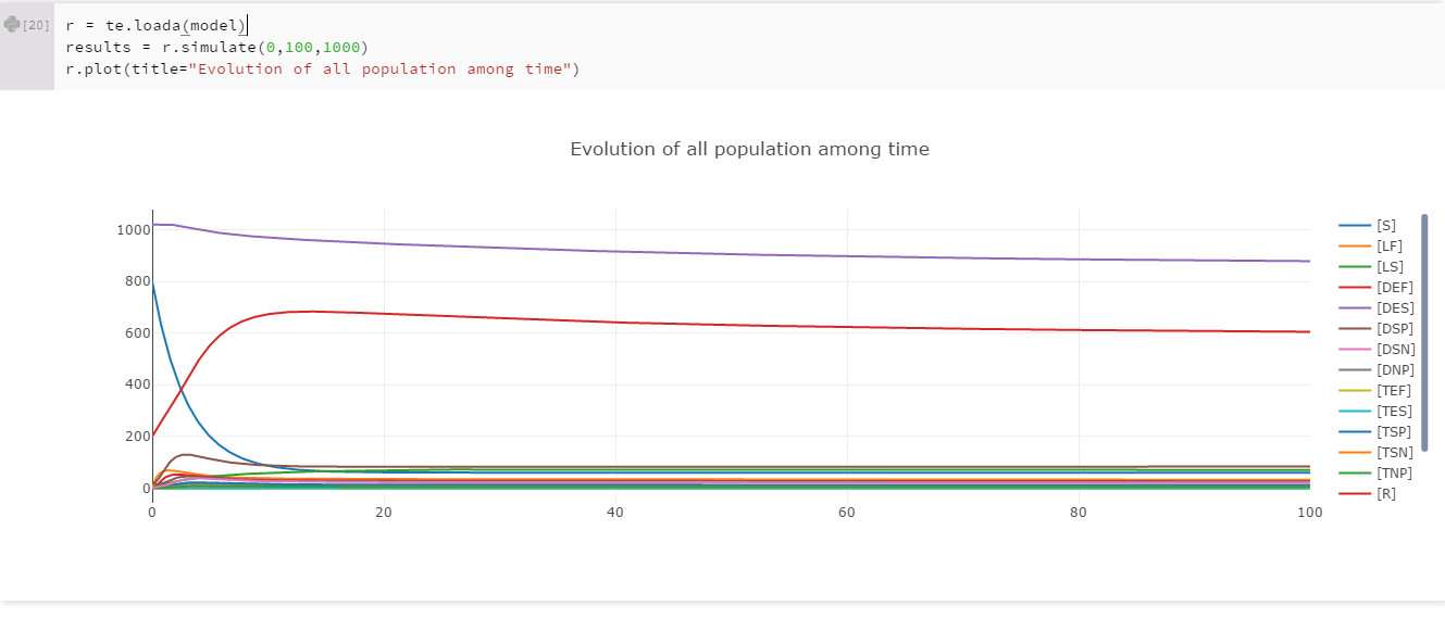
These first results showed us that the model seems good. We know that the infectiousness of smear positive diseased people (DSP) is really high. As we set an initial popupation of DSP to 20 (2% of the initial population), we expected that the disease spread to all the population. Nevertheless we didn't expected that the spreading would be that fast. In less than 15 years, more than 90% of the population is infected. The light purple curve represent the ALL population, which is simply the sum of the susceptible (S), recovered (R) and smear positive diseased (DSP) population. For further exploration of the model, we tried to see which paramter has an impact on the population decrease.
Running simulations with changing parameters
To show the impact of diagnosis parameters on the population, we ran some simulations with a range of variation in diagnosis parameters.
Diagnosis efficiency impact
The diagnosis efficiency was the first parameter we wanted to test its impact. As said before, it's modeled as the z variable and it's set to 2 initially. The simulation made it vary from 1 to 10 with a step of 1. After running the simulation, we got the following results:
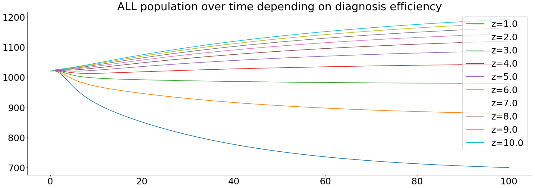
The orange curve represents the default value of the diagnosis efficiency. Knowing that we're use a value a little bit greater than in the paper (between 1.4 and 1.7). These results confirm that an increase in the diagnosis efficiency is one of the main keys to eliminate TB.
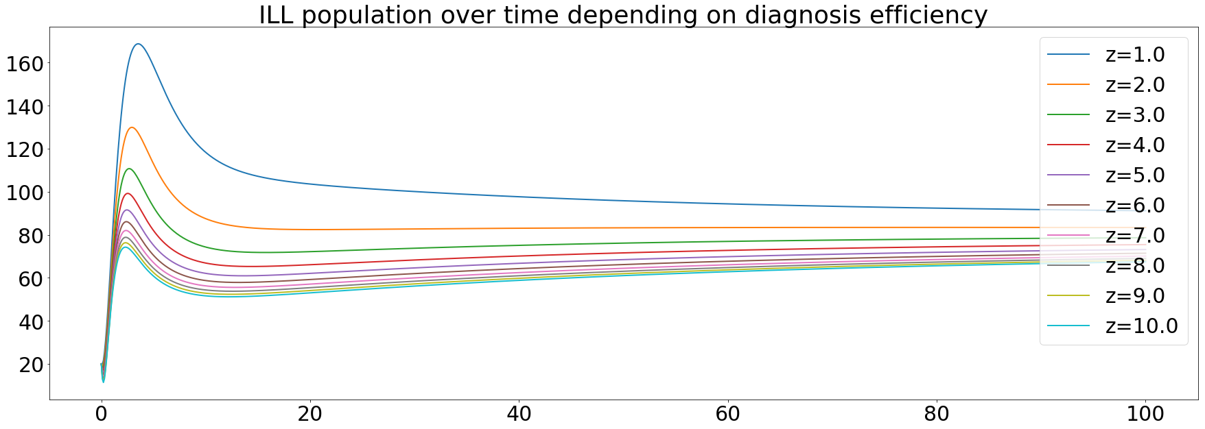
We can see that the ILL population depends on the diagnosis efficiency. That sounds logical since the more efficient the diagnosis is, the more the population will be treated.
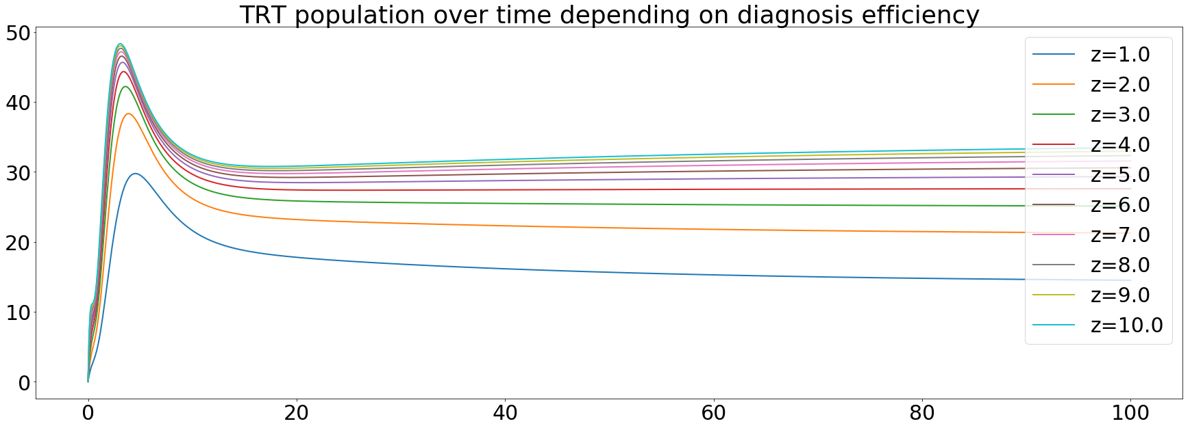
The treated population increases during the first 20 years then get stable. It can be explained by the fact that more people are being treated and the infectivity of TB begins to decrease after 20 years.
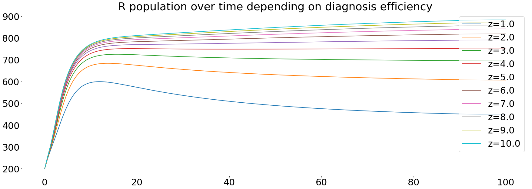
Finally, the recovered population, cured people with a chance of being re-infected, increases over time. Meaning that the diagnosis efficiency has a great impact on the capability of curing people from the tuberculosis.
After seeing these results, we wanted to see how the diagnosis of the different disease stages impact the model. In order to see that, we ran simulation with variation of the case detection rate of the different disease states, Xsp, Xsn and Xnp for smear positive disease, smear negative disease and non pulmonary disease respectively.
The most infective state of the disease is the smear positive one, we wanted to see if the diagnosis of this state should a bigger concern than the others. The initial value was set to 0.5, meaning that 50% of smear positive cases would be detected. The range in the simulation goes from 0.4 to 0.95, 40% to 95% respectively.
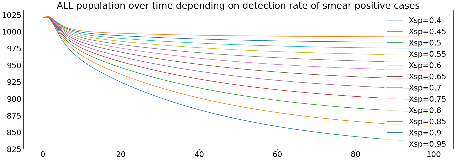
The results here are similar to the results obtained from the simulation of the impact of the diagnosis efficiency. The diagnosis of the smear positive state enable the stabilasation of the population 20 years after the marketing of the new diagnosis test with an efficiency of 95%. We will not look at all the differentpopulation, because the effect we wanted to see is the impact on the global population
The smear negative state of the disease is less infectious than the previous one, but it is still possible that a smear negative diseased personn infect a susceptible one. We ran the same simulation as before but with variation in the Xsn values.

As seen on the curves, the diagnosis efficiency of the smear negative state prevent from a total dying of the population caused by the tuberculosis, but we still get a decrease of the population by 200. The diagnosis of this state seems to be less effective than the smear positive state if we want to have a complete recovery of the population.
The last state of the disease is th non pulmonary. This one is less infective than the two other and the mortality rate is similar to the smear negative one. We also ran simulations of the impact of the diagnosis of this state, the same way than before.
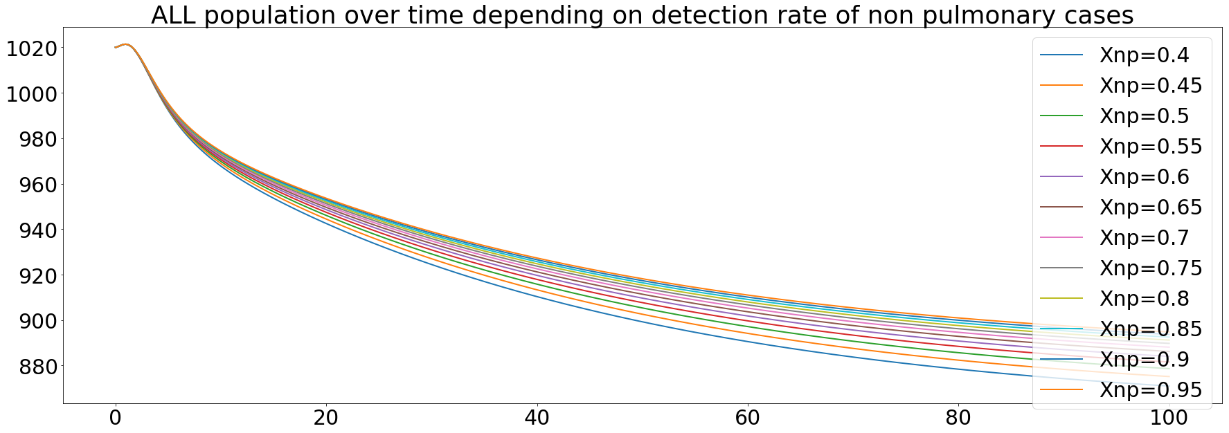
We observe the same behavior than the diagnosis of the smear negative state. This can be explained by the fact that in the model, we set the smear negative and the non pulmonary states to have the same mortality rates, based on the WHO data.
Using our model, we could see that the smear positive state has the biggest impact on the global population. Seeing this, we decided to concentrate our efforts on this state of the disease. We can resume the results of our simulations with the following graph.

On the above barplot, the y axis represents the final population after the simulations and the x axis the efficiency of the diagnosis, varying from 1 to 10. The red line represents the initial population set to 1020. We can see that with an increase of the diagnosis efficiency, the final population exceeds the initial population. Thereby, the tuberculosis spreading is stopping or at least is slower.