Team:Athens/Model
-

- People
MEDEA/Model ΜΕΔΕΑ
Modelling
Modelling
Overview
Alongside with our wet lab work, computational modelling of our MEDEA (Machine - Enhanced Directed Evolution of Aptamers) system has been proven to be crucial in order to establish a workflow for future applications. The main focus of our model has been to correlate the binding affinity of the evolved aptamers to the outcome of the selection module, namely the ability of our bacteria to survive under a given antibiotic concentration. In order to achieve that, we had to develop a single-cell kinetic model of the circuit, which enabled us to establish the rates at which a cell becomes resistant to the selection pressure, according to the Resistance Molecules it maintains internally.
Apart from the main models, as part of the design of our aptazyme, we used software to assess if there are conformational changes in the active center of the ribozyme. Specifically, we chose to use RNAfold and RNA Composer.
In the following sections we describe an outline of the aforementioned models and, most importantly, the thinking process we followed during their development. We hope they will serve as a helpful companion to anyone who wishes to use MEDEA in the future, and, as everything else in iGEM, open to recommendations and improvements from the SynBio community.
Pre-equation explanations
Assumptions:
1. The concentration of Arabinose (henceforth [Ara]) in the medium is staying constant.
Examining this claimUsing the Harvard Bionumbers database1, the average E. coli DH5α cell volume was set to be 1.1 μ\(\text{m}^3\) 2. Let's also consider a popular [Ara] used in the literature, which is quite small. For this claim, this should be 0.002% w/v, but in the final model, it will be just [Ara]. In the Toprak et al. version of the Morbidostat3, an OD of 0.15 to 0.2 is suggested. Let's consider the lower of the two, 0.15. While we will adjust our own preferred OD600 based on the CFU we observe at various ODs, for now lets use the "rule of thumb", which is that an OD600=1 is equal to 7*108 cells/mL of culture in LB broth4. That means that an OD600 of 0.15 would be 0.15*7*108 or 1.05 * 108 cells/mL of culture. Finally, since our plasmid is low copy in itself and the insert is quite large, we will assume that the copy number is less than 10, but for now, we will use 10. It follows that in low copy numbers, the threshold for [Ara] activation is smaller than in a higher copy number, because AraC has less places to bind. In our medium, we can easily calculate the concentration of arabinose as 0.024 grams in the 12 mL culture we are going to use and given Arabinose's Molecular Weight which is 150.13 g/mol, we can figure out that in our medium, we have 0.024/150.13 mol of Arabinose. Since the medium is constantly supplied, we will assume that Arabinose degradation is a term we can exclude. Next, using Avogadro's constant, we can easily calculate the number of molecules of Arabinose in our medium. Lastly, suppose that all of our bacteria have their Arabinose inducible promoters activated by AraC. Activating one AraC system in 1 bacterial cell requires 50 μM5 of inner [Ara], or (since n = C * V) 50 * 1.1 * 10-15 * 10-6 mol, since one μ\(\text{m}^3\) is 10-15 L and one μΜ is 10-6 M or mol/L. Since we have 12 * 1.05 * 108 cells in our culture, we will also multiply the number by that. Finally, we can figure out that in our medium we have about 9.627081969 * 1019 molecules of arabinose and all our bacterial cells together need 4.1732 * 1013 molecules of arabinose to activate all AraC systems. As such, all Arabinose dependent systems can be active at the same time (worst case scenario) and there would still be a lot of leftover Arabinose in the system. We also note that this assumption is one that is used in the literature plenty of times, as the aforementioned citations show.
On the intake of Arabinose:
First, we should note that we are using NEB DH5α cells and consulted their genome sequence data in order to figure out which Ara related genes they had endogenously6. For all genes that were not correctly annotated, we used BLAST to figure out their identity. They seem to have AraC (DNA binding transcriptional regulator), AraJ (MFS transporter, putative efflux pump), AraFGH (high affinity, low capacity transport of Arabinose). BLASTing the genome for AraE revealed its existence in an unannotated site in the genome. Arabinose is transported through the membrane either by AraE (proton cotransporter) or AraFGH (passive diffusion through pores) and is degraded by the AraBAD metabolic genes, as well as exported through AraJ.
In order to simplify this model, we will use only one mechanism of intake, named upt (uptake) and only one for degradation and diffusion, named deg (degradation). Great resources on the Arabinose operon and its regulation are the reviews here7,8. Transcription by the AraC controlled genes is turned on 1 minute after Arabinose induction, as stated here9 and is turned off about 3 minutes after Arabinose removal, presumably due to efflux10. In low arabinose concentrations, an all-or-none response is observed, which was first regarded as a graded response due to subpopulations of bacteria not being activated. However, when a higher Arabinose concentration is used, all cells are induced and a graded response is observed11.
On the activation by Arabinose:
Robert Schleif, an expert in AraC, provides a great picture to explain exactly how Arabinose functions in his essay: (https://biophysics.jhu.edu/directory/robert-schleif for more information about him)
Some iGEM attempts on AraBAD/AraC:
We would like to preface this part by saying that this is by no means an exhaustive list but merely some of our own iGEM bibliographical reference review. There have been multiple attempts to model the AraC proteins. One of the first publications to employ a synthetic biology perspective in the modelling of an inducible arabinose system is the one that was also used by iGEM UC Davis 2013, based on the supplementary information of that 2011 publication13. An even earlier attempt has been made in iGEM though, with the St. Andrews' team modelling the system as early as 2011. In this system, they assumed cellular concentration of arabinose to be the sum of diffusion of Arabinose (upt in our model), dissociation of Arabinose from araC minus the sum of association of Arabinose to AraC and the degradation of Arabinose (deg in our model). They used a normal Hill function for the transcription factor binding and calculated their theoretical protein production. Based on the following papers, they gathered the parameters needed for their model9,14–17, along with information they found on the registry. The UC Davis 2013 team used a Shea Ackers formulism18,19, employing the concept of the probability of an active complex, using data they obtained on Bionumbers and the publication they based their model on1,13. In the same year, the Imperial College London 2013 iGEM team tried to model the same system, which also resulted in a publication20. In their model, which is a bit simplified, they only model the transcription of their desired mRNA using a Hill function and the Arabinose concentration. They also assume that the bacteria carry the initial medium concentration of Arabinose. One of the teams that attempted to model the same promoter was iGEM Oxford 2015. Their key assumption is that AraC binding to arabinose happens on a faster time scale to transcription, which is a solid assumption overall. Using that assumption, they rid themselves on any need to incorporate AraC binding to Ara in their model, as it is not the limiting reaction and they only start the modelling from the limiting reaction onward. They used the following publications to obtain the necessary parameters21–26. Last but not least, Heidelberg 2017 also modelled Arabinose, assuming the external concentration of Arabinose remained constant, but they did not model the promoter, only the time needed to reach an equilibrium in Arabinose concentration for their PACE experiments.
Our AraBAD/AraC model:
We will follow a different formulation than most of the previous models, the one outlined in this paper10. We chose this model, as it accounts for the uptake of Arabinose, the receptors needed and their concentration, the bacterial growth and arabinose leakage. The model itself is described in the differential equations in the appropriate section of the Equations below.
STAR modelling:
The transcript produced by the inducible arabinose promoter PBAD is an operon constructed from two genes, the SmR gene, which was found on Snapgene's database and was found out to be aadA, a gene that confers resistance to Streptomycin and Spectinomycin27,28, as well as the KanR gene, which was also found on Snapgene's database and was revealed to be the aminoglycoside-O-phosphotransferase (APH)29,30. The catalytic activity of aadA is to attach an adenyl group in Streptomycin, using ATP. Diving deeper into its function, using the Salmonella enterica gene analogue331 and under the assumption that ATP is present in a much larger concentration than the antibiotic in the cell, we will use the KD of 0.5 μM332, which is a result of an in vitro experiment made using ITC, the best estimate we have found so far. As for the resistance to Kanamycin, it also uses ATP to add a phosphor group to Kanamycin. In the same vein as before, we will assume ATP to be far larger and constant. We will also ignore the use of GTP as a cosubstrate for the reaction, even though it has been shown to be superior33. We will also assume, as we did before, that Kanamycin is neutralized in a single reaction, so we can use the Kd found that was 18.2 μM34,35. Since conditional differential equations cannot be created, these parameters were not integrated in the final model and the total protein concentration of the antibiotic resistance genes was used as a surrogate.
It is now important to figure out a way to calculate the number of stable proteins in the single-cell model at any given time. Looking at our plasmid, pEKATI, the reader could notice the STAR Target module that is placed in front of the operon-like transcript. In short, as already described on our other pages, the STAR Target module will create a terminator hairpin, stopping transcription before the transcripts are actually fully produced and therefore no translation of the two antibiotic resistance proteins can occur. The only two ways for the transcripts to be formed is either a malfunction in the STAR Target, not creating the terminator hairpin and therefore allowing transcription to occur normally or the existence of the STAR molecule, which is an RNA complementary to one part of the sequence of the STAR target and binding to it allows transcription to proceed normally, by prohibiting the STAR target from creating the needed hairpin loop.
Therefore, two conditions must be established before the two antibiotic resistance genes are properly expressed. First, the concentration of Arabinose in the cell must exceed a critical conenctration, so that transcription can be activated and second, there must be enough of the STAR RNA to inhibit the creation of the STAR target terminator hairpin. The rest of the parameters, such as transcription rate and translation rate, as well as the respective degradation rates were extracted from the Bionumbers database or literature references1.
Our modelling of the STAR module is very much akin to the team that first introduced the STAR molecules in iGEM, iGEM Imperial College London 2016, in the sense of us also using strand-displacement computational techniques to obtain kinetic constants for the reversible reaction shown on the appropriate group of equations on the Equations section.
Modelling the aptazyme:
Many times have scientists attempted to model aptazymes and many of those attempts have been deemed successful, in both cell free systems36, computational studies37, models that have been proposed38, in vitro coupled with in silico studies39 as well as reviews written on the subject40. Our choice was made based on the model seemed the most robust to us, as in, accounting for the most parameters. In this case, this appears to be also a reversible-reaction Aptamer interaction with its binding target, along with a (kinetically fast) autocatalysis reaction.
Continuing on our main assumptions list, we detail the following, as further supported by the aforementioned arguments' analysis on the listed references:
- Only very few free (i.e. unbound) STAR molecules get bound to already-transcribed ("OFF transcription" mode) mRNA, free on the cell.
- Almost all STAR molecules remain bound to the SmR_KanR_mRNA after its transcription termination.
- The bound STAR:STAR_Target_RNA is considered to not degrade, because of the kinetically very fast reaction of its transcription continuation to the final product: SmR_KanR_mRNA.
- The Aptazyme:Ligand complex is also considered non-degradable for the same reason, i.e. it immediately gets catalyzed, releasing a STAR molecule.
Equations
First of all, we gather our model's equations as supported by the explanations above in relevant groups that get intertwined through at most two variables, for reasons that have to do with a quite technical matter that will appear further down, i.e. better decoupling of non-linearities: \[ \begin{equation} \begin{aligned} \text{DNA} &\rightarrow \text{Aptazyme} \\ \text{Aptazyme} &\rightarrow O \\ \text{Aptazyme} + \text{Ligand} &\rightleftharpoons \text{Aptazyme:Ligand} \\ \text{Aptazyme:Ligand} &\rightarrow \text{Catalyzed_Aptazyme:Ligand} + \text{STAR} \end{aligned} \end{equation}\tag{1} \] \[ \begin{equation} \begin{aligned} \text{DNA} &\rightarrow \text{Ligand_mRNA} \\ \text{Ligand_mRNA} &\rightarrow \text{Ligand} \\ \text{Ligand_mRNA} &\rightarrow O \\ \text{Ligand} &\rightarrow O \end{aligned} \end{equation}\tag{2} \] \[ \begin{equation} \begin{aligned} \text{DNA} + \text{Ara} &\rightarrow \text{STAR_Target_RNA}\ \ \ \text{(Note: p\(_{\text{BAD}}\) model)} \\ \text{STAR} + \text{STAR_Target_RNA} &\rightleftharpoons \text{STAR:STAR_Target_RNA} \\ \text{DNA} + \text{STAR:STAR_Target_RNA} &\rightarrow \text{SmR_KanR_mRNA} \\ \text{SmR_KanR_mRNA} &\rightarrow \text{SmR} \\ \text{SmR_KanR_mRNA} &\rightarrow \text{KanR} \\ \text{STAR} &\rightarrow O \\ \text{STAR_Target_RNA} &\rightarrow O \\ \text{SmR_KanR_mRNA} &\rightarrow O \\ \text{SmR} &\rightarrow O \\ \text{KanR} &\rightarrow O \end{aligned} \end{equation}\tag{3} \] Before we present the analytical equations, it is important to mention our naming conventions, so that an attentive reader may not get confused:
\(\beta\) are transcription rates, \(\alpha\) are degradation + dilution rates, \(k\) are translation (and other) rates
Now, we are ready to write the corresponding (non-linear) System of Differential Equations in the following form: \[ \begin{equation} \begin{aligned} \frac{d\left[\text{Aptazyme}\right]}{dt} &= \beta_\text{aptaz} - \alpha_\text{aptaz}\left[\text{Aptazyme}\right] - k_\text{f,bind}\left[\text{Aptazyme}\right]\left[\text{Ligand}\right] + k_\text{r,bind}\left[\text{Aptazyme:Ligand}\right] \\ \frac{d\left[\text{Ligand_mRNA}\right]}{dt} &= \beta_\text{lig_mRNA} - \alpha_\text{lig_mRNA}\left[\text{Ligand_mRNA}\right]\ \ \ \text{(decoupled equation)} \\ \frac{d\left[\text{Aptazyme:Ligand}\right]}{dt} &= k_\text{f,bind}\left[\text{Aptazyme}\right]\left[\text{Ligand}\right] - \left( k_\text{r,bind} + k_\text{catal} \right) \left[\text{Aptazyme:Ligand}\right] \\ \frac{d\left[\text{STAR}\right]}{dt} &= k_\text{catal} \left[\text{Aptazyme:Ligand}\right] - \alpha_\text{STAR}\left[\text{STAR}\right] - k_\text{f,star_targ}\left[\text{STAR}\right]\left[\text{STAR_Target_RNA}\right] \\ &+ k_\text{r,star_targ}\left[\text{STAR:STAR_Target_RNA}\right] \\ \frac{d\left[\text{STAR:STAR_Target_RNA}\right]}{dt} &= k_\text{f,star_targ}\left[\text{STAR}\right]\left[\text{STAR_Target_RNA}\right] \\ &- \left( k_\text{r,star_targ} + \beta_\text{SmR_KanR_mRNA} \right)\cdot \left[\text{STAR:STAR_Target_RNA}\right] \\ \frac{d\left[\text{SmR_KanR_mRNA}\right]}{dt} &= \beta_\text{SmR_KanR_mRNA} \left[\text{STAR:STAR_Target_RNA}\right] - \alpha_\text{SmR_KanR_mRNA} \left[\text{SmR_KanR_mRNA}\right] \\ \frac{d\left[\text{SmR}\right]}{dt} &= k_\text{SmR} \left[\text{SmR_KanR_mRNA}\right] - \alpha_\text{SmR} \left[\text{SmR}\right] \\ \frac{d\left[\text{KanR}\right]}{dt} &= k_\text{KanR} \left[\text{SmR_KanR_mRNA}\right] - \alpha_\text{KanR} \left[\text{KanR}\right] \\ \frac{d\left[\text{Ligand}\right]}{dt} &= k_\text{lig}\left[\text{Ligand_mRNA}\right] - \alpha_\text{lig}\left[\text{Ligand}\right] - k_\text{f,bind}\left[\text{Aptazyme}\right]\left[\text{Ligand}\right] + k_\text{r,bind}\left[\text{Aptazyme:Ligand}\right] \\ \frac{d\left[\text{STAR_Target_RNA}\right]}{dt} &= u_\text{star_targ_RNA}(t) \left[\text{SmR_KanR_mRNA}\right] - k_\text{f,star_targ} \left[\text{STAR}\right]\left[\text{STAR_Target_RNA}\right] \\ &- k_\text{r,star_targ} \left[\text{STAR:STAR_Target_RNA}\right] - \alpha_\text{star_targ_RNA} \left[\text{STAR_Target_RNA}\right] \end{aligned} \end{equation} \] with \( K_d = \frac{k_\text{r,bind}}{k_\text{f,bind}}\Leftrightarrow k_\text{r,bind} = K_d\cdot k_\text{f,bind} \)
Continuing to the pBAD model of the AraBAD/AraC model, where \(a(t)\) is the internal arabinose concentration, \(N(t)\) is the number of AraE molecules, and \(n(t)\) is the number of AraE_mRNA molecules: \[ \begin{equation} \begin{aligned} u_\text{star_targ_RNA}(t) &= u_\text{0,star_targ_RNA} + (u_\text{max,star_targ_RNA} - u_\text{0,star_targ_RNA})\cdot \frac{a^3(t)}{K_a^3+a^3(t)} \\ \frac{da(t)}{dt} &= V_\text{upt}\cdot N(t) - \alpha_\text{ara}\cdot a(t) \\ V_\text{upt} &= V_\text{max}\cdot \frac{a_\text{ex}}{K_m+a_\text{ex}} \\ \frac{dn(t)}{dt} &= u_e(t) - \alpha_\text{AraE_mRNA}\cdot n(t) \\ u_e(t) &= u_\text{0,e} + (u_\text{max,e} - u_\text{0,e})\cdot \frac{a^3(t)}{K_a^3+a^3(t)} \\ \frac{dN(t)}{dt} &= \mu_e\cdot n(t) - \alpha_\text{AraE}\cdot N(t) \end{aligned} \end{equation} \] Therefore, the unknown time functions to be modelled are the following: \[ \left[\text{Aptazyme}\right],\ \left[\text{Ligand_mRNA}\right],\ \left[\text{Ligand}\right],\ \left[\text{Aptazyme:Ligand}\right],\ \left[\text{STAR}\right],\ \left[\text{STAR_Target_RNA}\right],\ \left[\text{STAR:STAR_Target_RNA}\right], \] \[ \left[\text{SmR_KanR_mRNA}\right],\ \left[\text{SmR}\right],\ \left[\text{KanR}\right],\ a(t),\ n(t),\ N(t) \]Parameters
Parameter Description Value from Literature Value used Reference \(\beta_\text{aptaz}\) Aptazyme constitutive promoter (CAT) transcription rate ~0.5 RPU 0.5 RPU https://jbioleng.biomedcentral.com/articles/10.1186/1754-1611-3-4 \(\beta_\text{Ligand_mRNA}\) Ligand_mRNA constitutive promoter (J23111) transcription rate 0.58 RPU 0.58 RPU https://peerj.com/articles/5862.pdf \(\beta_\text{SmR_KanR_mRNA}\) Rate of transcription continuation 190.0 \(\text{min}^{-1}\) 200.0 \(\text{min}^{-1}\) https://bionumbers.hms.harvard.edu/files/Kinetic%20parameters%20of%20open-complex%20formation.pdf , https://onlinelibrary.wiley.com/doi/abs/10.1111/j.1574-6976.2010.00226.x \(\alpha_\text{aptaz}\) Degradation + Dilution rate of Aptazyme 0.17 \(\text{min}^{-1}\) 0.17 \(\text{min}^{-1}\) https://ora.ox.ac.uk/objects/uuid:78bf0e95-ae8d-4ccd-af38-bc4b309e7ca7/download_file?file_format=pdf&safe_filename=Papachristodoulou%2Bet%2Bal%252C%2BFrequency%2Bdomain%2Banalysis%2Bof%2Bsmall%2Bnon-coding%2BRNAs%2Bshows%2Bsumming%2Bjunction-like%2Bbehaviour.pdf&type_of_work=Conference+item \(\alpha_\text{STAR}\) Degradation + Dilution rate of free STAR mRNA 0.17 \(\text{min}^{-1}\) 0.17 \(\text{min}^{-1}\) https://ora.ox.ac.uk/objects/uuid:78bf0e95-ae8d-4ccd-af38-bc4b309e7ca7/download_file?file_format=pdf&safe_filename=Papachristodoulou%2Bet%2Bal%252C%2BFrequency%2Bdomain%2Banalysis%2Bof%2Bsmall%2Bnon-coding%2BRNAs%2Bshows%2Bsumming%2Bjunction-like%2Bbehaviour.pdf&type_of_work=Conference+item \(\alpha_\text{SmR_KanR_mRNA}\) Degradation + Dilution rate of SmR_KanR_mRNA 0.17 \(\text{min}^{-1}\) 0.17 \(\text{min}^{-1}\) https://ora.ox.ac.uk/objects/uuid:78bf0e95-ae8d-4ccd-af38-bc4b309e7ca7/download_file?file_format=pdf&safe_filename=Papachristodoulou%2Bet%2Bal%252C%2BFrequency%2Bdomain%2Banalysis%2Bof%2Bsmall%2Bnon-coding%2BRNAs%2Bshows%2Bsumming%2Bjunction-like%2Bbehaviour.pdf&type_of_work=Conference+item \(\alpha_\text{star_targ_RNA}\) Degradation + Dilution rate of STAR_Target_RNA 0.17 \(\text{min}^{-1}\) 0.17 \(\text{min}^{-1}\) https://ora.ox.ac.uk/objects/uuid:78bf0e95-ae8d-4ccd-af38-bc4b309e7ca7/download_file?file_format=pdf&safe_filename=Papachristodoulou%2Bet%2Bal%252C%2BFrequency%2Bdomain%2Banalysis%2Bof%2Bsmall%2Bnon-coding%2BRNAs%2Bshows%2Bsumming%2Bjunction-like%2Bbehaviour.pdf&type_of_work=Conference+item \(\alpha_\text{SmR}\) Dilution + Degradation rate of SmR protein 0.03 \(\text{min}^{-1}\) 0.03 \(\text{min}^{-1}\) https://ora.ox.ac.uk/objects/uuid:78bf0e95-ae8d-4ccd-af38-bc4b309e7ca7/download_file?file_format=pdf&safe_filename=Papachristodoulou%2Bet%2Bal%252C%2BFrequency%2Bdomain%2Banalysis%2Bof%2Bsmall%2Bnon-coding%2BRNAs%2Bshows%2Bsumming%2Bjunction-like%2Bbehaviour.pdf&type_of_work=Conference+item \(\alpha_\text{KanR}\) Dilution + Degradation rate of KanR protein 0.03 \(\text{min}^{-1}\) 0.03 \(\text{min}^{-1}\) https://ora.ox.ac.uk/objects/uuid:78bf0e95-ae8d-4ccd-af38-bc4b309e7ca7/download_file?file_format=pdf&safe_filename=Papachristodoulou%2Bet%2Bal%252C%2BFrequency%2Bdomain%2Banalysis%2Bof%2Bsmall%2Bnon-coding%2BRNAs%2Bshows%2Bsumming%2Bjunction-like%2Bbehaviour.pdf&type_of_work=Conference+item \(\alpha_\text{lig_mRNA}\) Degradation + Dilution rate of Ligand_mRNA (here: CRP_mRNA) 0.17 \(\text{min}^{-1}\) 0.17 \(\text{min}^{-1}\) https://ora.ox.ac.uk/objects/uuid:78bf0e95-ae8d-4ccd-af38-bc4b309e7ca7/download_file?file_format=pdf&safe_filename=Papachristodoulou%2Bet%2Bal%252C%2BFrequency%2Bdomain%2Banalysis%2Bof%2Bsmall%2Bnon-coding%2BRNAs%2Bshows%2Bsumming%2Bjunction-like%2Bbehaviour.pdf&type_of_work=Conference+item \(\alpha_\text{lig}\) Dilution + Degradation rate of Ligand (here: CRP) 0.03 \(\text{min}^{-1}\) 0.03 \(\text{min}^{-1}\) https://ora.ox.ac.uk/objects/uuid:78bf0e95-ae8d-4ccd-af38-bc4b309e7ca7/download_file?file_format=pdf&safe_filename=Papachristodoulou%2Bet%2Bal%252C%2BFrequency%2Bdomain%2Banalysis%2Bof%2Bsmall%2Bnon-coding%2BRNAs%2Bshows%2Bsumming%2Bjunction-like%2Bbehaviour.pdf&type_of_work=Conference+item \(k_\text{SmR}\) SmR_mRNA translation rate (17.6 sec calculated) 3.41 \(\text{min}^{-1}\) Calculated from https://bionumbers.hms.harvard.edu/bionumber.aspx?id=109043&ver=3&trm=translation+e+coli+&org= and our sequence lengths \(k_\text{KanR}\) KanR_mRNA translation rate (18.13 sec calculated) 3.31 \(\text{min}^{-1}\) Calculated from https://bionumbers.hms.harvard.edu/bionumber.aspx?id=109043&ver=3&trm=translation+e+coli+&org= and our sequence lengths \(k_\text{lig}\) Ligand_mRNA (here: CRP_mRNA) translation rate (16.49 sec calculated) 3.64 \(\text{min}^{-1}\) Calculated from https://bionumbers.hms.harvard.edu/bionumber.aspx?id=109043&ver=3&trm=translation+e+coli+&org= and our sequence lengths \(k_\text{catal}\) Aptazyme autocatalysis rate 100 \(\text{min}^{-1}\) 100 \(\text{min}^{-1}\) https://www.mdpi.com/1420-3049/22/1/78/htm \(k_\text{f,star_targ}\) Forward reaction rate of the STAR binding to STAR_Target_RNA N/A 0.9 Calculated using strand displacement related techniques from Control of DNA Strand Displacement Kinetics Using Toehold Exchange \(k_\text{r,star_targ}\) Reverse reaction rate of the STAR binding to STAR_Target_RNA N/A 0.3 Calculated using strand displacement related techniques from Control of DNA Strand Displacement Kinetics Using Toehold Exchange \(k_\text{f,bind}\) Forward reaction rate of the Aptamer dissociation equilibrium \(\approx 10^{-2}\) \(10^{-2}\) Calculated using kinetic extrapolation with information from https://pubs.rsc.org/en/content/articlelanding/2019/an/c9an01247h/ and https://www.ncbi.nlm.nih.gov/pmc/articles/PMC4562382/ \(k_\text{r,bind}\) Reverse reaction rate of the Aptamer dissociation equilibrium \(\approx 1.25\cdot 10^{-9} \) \( 1.25\cdot 10^{-9} \) Calculated using \(k_\text{f,bind}\) and the below referenced \(K_d\) from the equation referred on the "Equations" section \(K_d\) Aptazyme reversible reaction dissociation equilibrium constant 125 nM 125 nM CRP Aptamer chosen from the commercially available on the Aptagen Index
Note 1: In addition, we utilized the parameters described for the Arabinose AraBAD/AraC system, as mentioned before, from Single Cell Kinetics of Phenotypic Switching in the Arabinose Utilization System of E. coli supplementary information sheets.
Note 2: By "value used" in the above table we mean that certain applicable values were modified according to a batch of simulations, expected results, and automated loop parameter modifications, in order to simulate more accurately our whole-system effect. Therefore, those changed values can be described as "best-fit" to the simulations performed.
AraBAD Results
Our model study included an AraBAD/AraC model as a sub-model, as described extensively in the above sections, with a specific emphasis for a better model than those currently used in the past iGEM years. Hereby, we exhibit our graphic results along with very short comments on them:
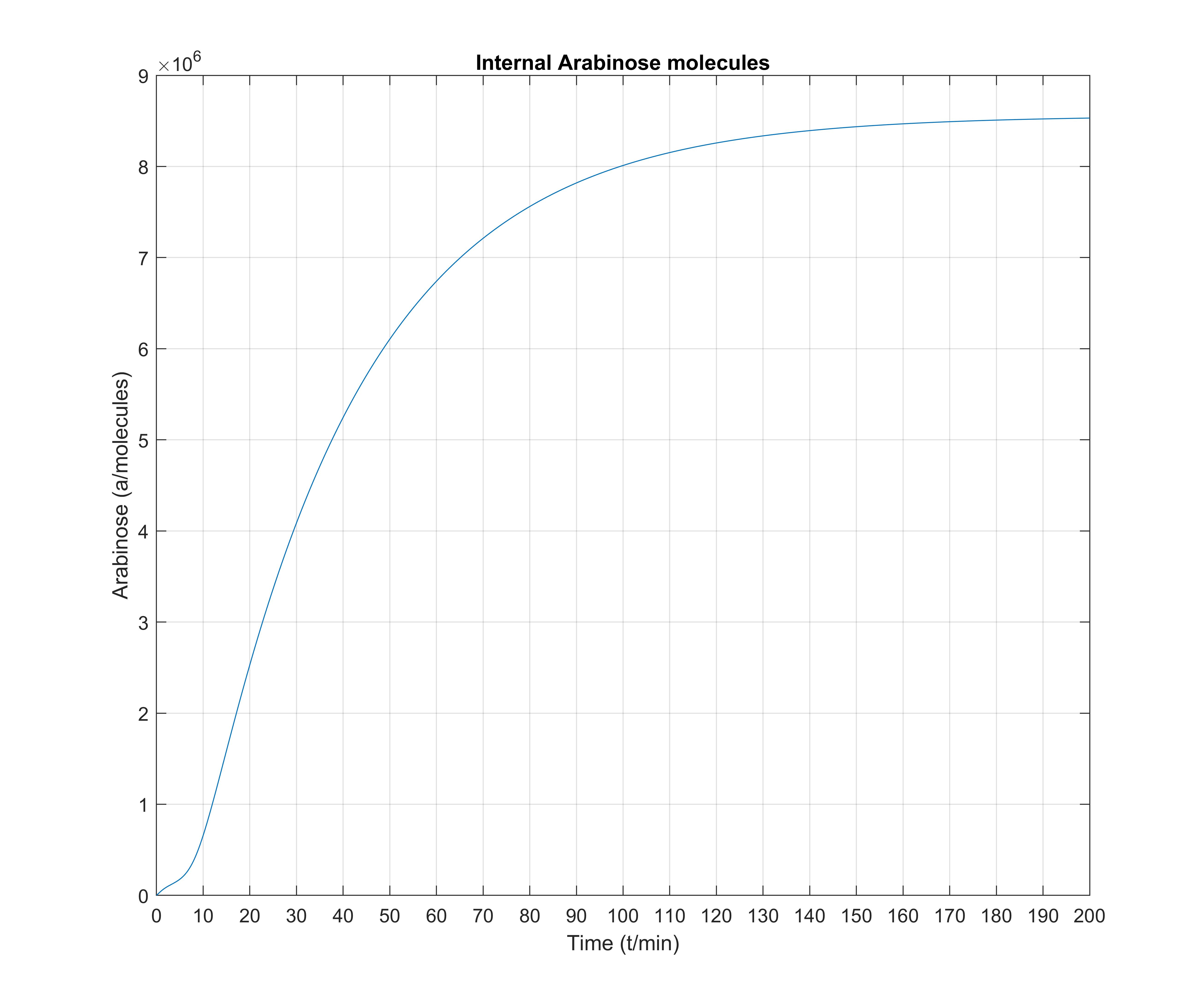
One notable observation is that, even though arabinose slowly and steadily enters the cell through the transporters, \(P_\text{BAD}\) total activation happens very fast, rising to \(\approx 90\%\) within at most 5 minutes, whereas internal arabinose molecules settle at about 180 minutes. Therefore, it seems that while the model is a gradient model, the all or nothing response to Arabinose often observed in the literature is a result of the quick activation of transcription.
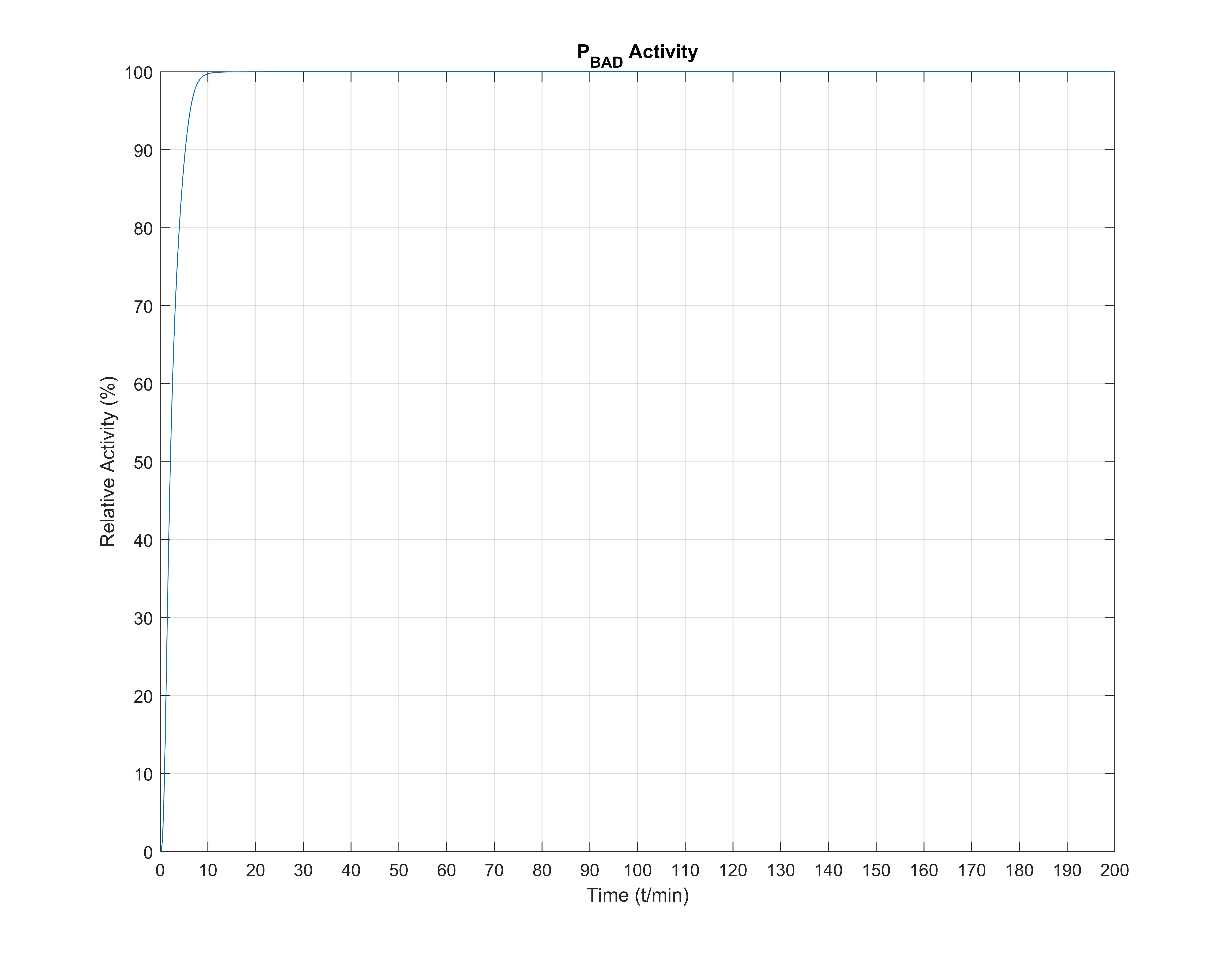
In the above graphic figure we denote that AraE (transporters) and internal arabinose molecules follow almost the same time distribution, a very logical fact indeed for cell survival in arabinose environments, for which the original AraBAD/AraC system was found out for.
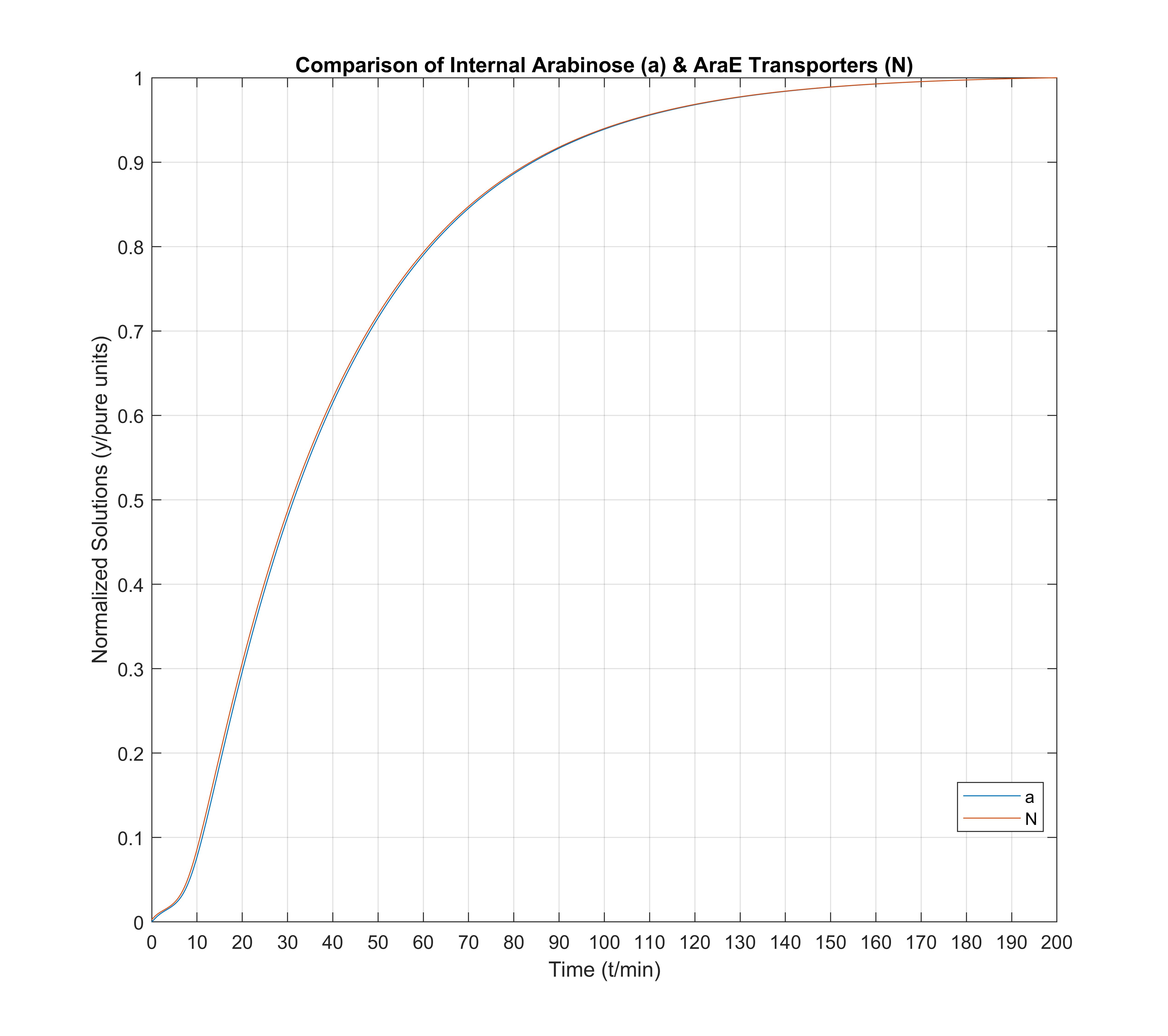
Finally, in this last figure we view a comparison between the arabinose transporter (AraE) mRNA and the internal arabinose molecules. We note especially that a minuscule amount of internal arabinose existence is more than enough to immediately activate the arabinose transport system. AraE_mRNA "acts fast", as expected, and gets the cell ready for arabinose absorption from the environment though transport quickly.
Note for the three above figures: all these are depicted normalized to unitary units, so that comparisons between graph shapes can easily be made.
System Results
First of all, in order to better visualize the whole system, and for the reinforcement of the understanding of such a complex system, we created a SimBiology model description, which resulted in the following visualization, that will help readers realize the exact reactions taking place in the model:
There, we attempted many different simulations by altering the simulations settings. Stochastic modelling, unfortunately, cannot be applied currently with non-MassAction kinetic laws (such as the approximate Hill Functions that the Arabinose model incurs), therefore we contacted MathWorks about this fact, made an official proposal, and got a response that our request will be taken into consideration for future research work and integration into the program. This will allow many other iGEM teams to take advantage of more accurate (by including probability distributions, thus increasing stochasticity of the system and approaching real-time conditions modelling) predictions and results, thus accelerating the development of much more accurate simulations. Therefore, we hope that the impact of our proposal will be significant on the whole computational biology community.
However, we noticed that for some specific parameter values close to our final chosen ones presented in the aforementioned table, the system behaves rather oddly, including some oscillations in the beginning of the simulation, that after careful consideration we attributed to the misrepresentation of correct choice of time steps between each iteration, as well as inadequate relative tolerance calculations in the simulation algorithms, and therefore decided to use Wolfram Mathematica for these specific values. Wolfram Mathematica is a computer program tailored for mathematical calculations that is able to solve systems of non-linear differential equations with more accuracy, which is desirable for a certain set of parameters, for which numerical instability is observed, even in Matlab's stiff system-of-differential-equations solvers, e.g. ode15s.
Furthermore, in order to make sure, and characterize our time response parameters, such as the time taken for the system to fully respond (the rise time), as well as for making sure that there are no inherent instabilities present on our solutions, we studied the steady-state solutions of our equations, partly through a theoretical point of view and partly (for the unsolvable part) through numerical solution, again utilizing both Matlab and Mathematica.
According to theoretical mathematical analysis, the following relations hold for the steady-state quantities: \[ [\text{Ligand_mRNA}] = \frac{\beta_\text{lig_mRNA}}{\alpha_\text{lig_mRNA}} \] \[ [\text{SmR_KanR_mRNA}] = \frac{\beta_\text{SmR_KanR_mRNA}}{\alpha_\text{SmR_KanR_mRNA}}\cdot [\text{STAR:STAR_Target_RNA}] \] \[ [\text{SmR}] = \frac{k_\text{SmR}}{\alpha_\text{SmR}}\cdot \frac{\beta_\text{SmR_KanR_mRNA}}{\alpha_\text{SmR_KanR_mRNA}}\cdot [\text{STAR:STAR_Target_RNA}] \] \[ [\text{KanR}] = \frac{k_\text{KanR}}{\alpha_\text{KanR}}\cdot \frac{\beta_\text{SmR_KanR_mRNA}}{\alpha_\text{SmR_KanR_mRNA}}\cdot [\text{STAR:STAR_Target_RNA}] \]
Then, we tried a batch of different parameters on our differential equation system, and observed that initially the variations of Antibiotic Resistance Molecules SmR and KanR were not as viewable (as a function of \(K_d\)) as we would like them to be, although big changes were observed between certain parameter values. This further proved our intuition for the high sensitivity of our system to certain parameters, such as the rate of transcription of the CRP mRNA, and the rate of transcription of the Aptazyme, both of which greatly affect the number of the resultant ARM molecules. This was exactly what showed the need for a slight modification of the wet lab design perspective, providing feedback for our method, in that the model suggested that weaker promoters be used for both the Aptazyme and the Ligand. With these modifications, we obtained the following time responses on our system, where we have also included the normalized values of all molecule numbers on a separate figure, in order to compare and contrast the shapes of the relevant quantities:
Finally, a 3D graph was constructed so that the time- and \(K_d\)-dependent evolution is depicted appropriately and at a glance, according to a large amount of simulation data we obtained through hours of computing:

The above 3D graph figure verifies our system works according to the model, because it depicts a strictly decreasing (math terminology) function of \(\text{SmR}\) with \(K_d\), exactly as desired, meaning that when the \(K_d\) increases (worse aptamer), the resulting \(\text{SmR}\) molecules (available to the cell) decrease, therefore the bacterium's resistance to antibiotics gradually decreases, leading it (under appropriate external antibiotic concentration) to cell death, as planned when unfit for Directed Evolution to work. Also, we notice that this graph when projected to the yz-plane (look at the silouette in the left plane for \( t=200 \text{min} \) ) gets saturated at some \(K_d\approx 10^{-8.5} M\) which means that it cannot work as accurately for very, very good aptazymes, but instead further promoter strengths (mainly) need to be more exactly adjusted in order to obtain a probably more desired result.
We, hereby, also present, for completeness the analytical derivation of the steady-state result for the Aptazyme:Ligand complex quantity from Wolfram Mathematica symbolic calculations, as this is the most important intermediate in our system, and one that affects all further gene expressions, introducing the dependence on the aptamer dissociation constant \(K_d\) through the relation of the quantities \(k_\text{f,bind}\), \(k_\text{r,bind}\) (as described in the "Equations" section):

- Milo, R., Jorgensen, P., Moran, U., Weber, G. & Springer, M. BioNumbers The database of key numbers in molecular and cell biology. Nucleic Acids Res. (2009). doi:10.1093/nar/gkp889
- Kubitschek, H. E. & Friske, J. A. Determination of bacterial cell volume with the Coulter Counter. J. Bacteriol. (1986). doi:10.1128/jb.168.3.1466-1467.1986
- Toprak, E. et al. Building a morbidostat: An automated continuous-culture device for studying bacterial drug resistance under dynamically sustained drug inhibition. Nat. Protoc. (2013). doi:10.1038/nprot.2013.021
- Sezonov, G., Joseleau-Petit, D. & D'Ari, R. Escherichia coli physiology in Luria-Bertani broth. J. Bacteriol. (2007). doi:10.1128/JB.01368-07
- Megerle, J. A., Fritz, G., Gerland, U., Jung, K. & Rädler, J. O. Timing and dynamics of single cell gene expression in the arabinose utilization system. Biophys. J. (2008). doi:10.1529/biophysj.107.127191
- Anton, B. P. & Raleigh, E. A. Complete genome sequence of NEB 5α-alpha, a derivative of Escherichia coli K-12 DH5αα. Genome Announc. (2016). doi:10.1128/genomeA.01245-16
- Schleif, R. Regulation of the L-arabinose operon of Escherichia coli. Trends in Genetics (2000). doi:10.1016/S0168-9525(00)02153-3
- Marschall, L., Sagmeister, P. & Herwig, C. Tunable recombinant protein expression in E. coli: promoter systems and genetic constraints. Applied Microbiology and Biotechnology (2017). doi:10.1007/s00253-016-8045-z
- Guzman, L. M., Belin, D., Carson, M. J. & Beckwith, J. Tight regulation, modulation, and high-level expression by vectors containing the arabinose P(BAD) promoter. J. Bacteriol. (1995). doi:10.1128/jb.177.14.4121-4130.1995
- Fritz, G. et al. Single cell kinetics of phenotypic switching in the arabinose utilization system of E. coli. PLoS One (2014). doi:10.1371/journal.pone.0089532
- Afroz, T., Biliouris, K., Kaznessis, Y. & Beisel, C. L. Bacterial sugar utilization gives rise to distinct single-cell behaviours. Mol. Microbiol. (2014). doi:10.1111/mmi.12695
- Schleif, R. AraC protein: A love-hate relationship. BioEssays (2003). doi:10.1002/bies.10237
- Tamsir, A., Tabor, J. J. & Voigt, C. A. Robust multicellular computing using genetically encoded NOR gates and chemical 'wiresg'. Nature (2011). doi:10.1038/nature09565
- Hendrickson, W. & Schleif, R. F. Regulation of the Escherichia coli l-arabinose operon studied by gel electrophoresis DNA binding assay. J. Mol. Biol. (1984). doi:10.1016/0022-2836(84)90241-9
- Kootstra, A. M. J., Mosier, N. S., Scott, E. L., Beeftink, H. H. & Sanders, J. P. M. Differential effects of mineral and organic acids on the kinetics of arabinose degradation under lignocellulose pretreatment conditions. Biochem. Eng. J. (2009). doi:10.1016/j.bej.2008.09.004
- Davidson, C. J., Narang, A. & Surette, M. G. Integration of transcriptional inputs at promoters of the arabinose catabolic pathway. BMC Syst. Biol. (2010). doi:10.1186/1752-0509-4-75
- Alon, U. An introduction to systems biology: Design principles of biological circuits. An Introduction to Systems Biology: Design Principles of Biological Circuits (2006).
- Ackers, G. K., Johnson, A. D. & Shea, M. A. Quantitative model for gene regulation by λ phage repressor. Proc. Natl. Acad. Sci. U. S. A. (1982). doi:10.1073/pnas.79.4.1129
- Bintu, L. et al. Transcriptional regulation by the numbers: Models. Current Opinion in Genetics and Development (2005). doi:10.1016/j.gde.2005.02.007
- Kelwick, R. et al. A forward-design approach to increase the production of poly-3-hydroxybutyrate in genetically engineered escherichia coli. PLoS One (2015). doi:10.1371/journal.pone.0117202
- Liang, S. T., Ehrenberg, M., Dennis, P. & Bremer, H. Decay of rpIN and lacZ mRNA in Escherichia coli. J. Mol. Biol. (1999). doi:10.1006/jmbi.1999.2710
- Proshkin, S., Rachid Rahmouni, A., Mironov, A. & Nudler, E. Cooperation between translating ribosomes and RNA polymerase in transcription elongation. Science (80-. ). (2010). doi:10.1126/science.1184939
- Sourjik, V. & Berg, H. C. Functional interactions between receptors in bacterial chemotaxis. Nature (2004). doi:10.1038/nature02406
- Salto, R., Delgado, A., Michán, C., Marqués, S. & Ramos, J. L. Modulation of the function of the signal receptor domain of XylR, a member of a family of prokaryotic enhancer-like positive regulators. J. Bacteriol. (1998).
- Selinger, D. W., Saxena, R. M., Cheung, K. J., Church, G. M. & Rosenow, C. Global RNA half-life analysis in Escherichia coli reveals positional patterns of transcript degradation. Genome Res. (2003). doi:10.1101/gr.912603
- Andersen, J. B. et al. New unstable variants of green fluorescent protein for studies of transient gene expression in bacteria. Appl. Environ. Microbiol. (1998).
- Clark, N. C., Olsvik, Ø., Swenson, J. M., Spiegel, C. A. & Tenover, F. C. Detection of a streptomycin/spectinomycin adenylyltransferase gene (aadA) in Enterococcus faecalis. Antimicrob. Agents Chemother. (1999).
- Magrini, V., Creighton, C., White, D., Hartzell, P. L. & Youderian, P. The aadA gene of plasmid R100 confers resistance to spectinomycin and streptomycin in Myxococcus xanthus. J. Bacteriol. (1998).
- Cohen, S. N., Chang, A. C. & Hsu, L. Nonchromosomal antibiotic resistance in bacteria: genetic transformation of Escherichia coli by R-factor DNA. Proc. Natl. Acad. Sci. U. S. A. (1972). doi:10.1073/pnas.69.8.2110
- Oka, A., Sugisaki, H. & Takanami, M. Nucleotide sequence of the kanamycin resistance transposon Tn903. J. Mol. Biol. (1981). doi:10.1016/0022-2836(81)90438-1
- Stern, A. L. et al. Structural mechanism of AadA, a dual-specificity aminoglycoside adenylyltransferase from Salmonella enterica. J. Biol. Chem. (2018). doi:10.1074/jbc.RA118.003989
- Chen, Y., Näsvall, J., Wu, S., Andersson, D. I. & Selmer, M. Structure of AadA from Salmonella enterica: A monomeric aminoglycoside (3'')(9) adenyltransferase. Acta Crystallogr. Sect. D Biol. Crystallogr. (2015). doi:10.1107/S1399004715016429
- Stogios, P. J. et al. Structure-guided optimization of protein kinase inhibitors reverses aminoglycoside antibiotic resistance. Biochem. J. (2013). doi:10.1042/BJ20130317
- Lallemand, P. et al. Transient kinetics of aminoglycoside phosphotransferase(3′)-IIIa reveals a potential drug target in the antibiotic resistance mechanism. FEBS Lett. (2012). doi:10.1016/j.febslet.2012.10.027
- Kaul, M., Barbieri, C. M., Srinivasan, A. R. & Pilch, D. S. Molecular Determinants of Antibiotic Recognition and Resistance by Aminoglycoside Phosphotransferase (3′)-IIIa: A Calorimetric and Mutational Analysis. J. Mol. Biol. (2007). doi:10.1016/j.jmb.2007.02.103
- Kobori, S., Ichihashi, N., Kazuta, Y., Matsuura, T. & Yomo, T. Kinetic analysis of aptazyme-regulated gene expression in a cell-free translation system: Modelling of ligand-dependent and -independent expression. RNA (2012). doi:10.1261/rna.032748.112
- Chen, X. & Ellington, A. D. Design principles for ligand-sensing, conformation-switching ribozymes. PLoS Comput. Biol. (2009). doi:10.1371/journal.pcbi.1000620
- Carothers, J. M., Goler, J. A., Juminaga, D. & Keasling, J. D. Model-driven engineering of RNA devices to quantitatively program gene expression. Science (80-. ). (2011). doi:10.1126/science.1212209
- McKeague, M., Wang, Y. H. & Smolke, C. D. In Vitro Screening and in Silico Modelling of RNA-Based Gene Expression Control. ACS Chem. Biol. (2015). doi:10.1021/acschembio.5b00518
- Jang, S., Jang, S., Yang, J., Seo, S. W. & Jung, G. Y. RNA-based dynamic genetic controllers: development strategies and applications. Current Opinion in Biotechnology (2018). doi:10.1016/j.copbio.2017.10.005