Team:Oxford/Model/Design

Modelling Design

Part I: Dynamic Expression vs. Constitutive Expression of Endolysin

To build our genetic circuit in vitro, we first needed to establish whether expression of endolysin in the ProQuorum system would be constitutive or regulated.

Assumptions

• Each L. reuteri cell produces the theoretically predicted concentration of endolysin.
• When endolysin production is induced in the dynamic expression system, all cells begin synthesis simultaneously.

Kinetic Rates

To inform our decision, we built mathematical models of both forms of expression using kinetic data constants derived from our wet lab work.

a) Concentration of endolysin produced per L. reuteri cell required for lysis of C. difficile cells estimated from experimental killing assay data of surrogate target bacterium B. subtilis (further detailed in the Supplementary Materials page.)

Endolysin Concentration Produced per L. reuteri cell /M CFU -1
0.00465

b) Stress on L. reuteri growth rate due to constitutive expression of CD27L endolysin:

Type of L. reuteri	Doubling time /hr	Growth Rate (ln 2/Doubling Time) /hr -1
Wild Type	0.548	1.26
Consitutively Expressing CD27L Endolysin	9.08	0.76

Differential Equations

Species Key:

Process Modelled	Differential Equation 1	Explanation 1	Differential Equation 2	Explanation 2
Logistic Growth Model of L. reuteri - Constitutive Expression	$$\frac {dC}{dt} = r_{stressed} \times C \times (1- \frac {C}{N_{lr}})$$	Endolysin is being expressed constitutively.	N/A	N/A
Logistic Growth Model of L. reuteri - Dynamic Expression	$$\frac {dR_{1}}{dt} = r_{wildtype} \times R \times (1- \frac {R}{N_{lr}})$$	If endolysin is not being expressed.	$$\frac {dR_{2}}{dt} = r_{stressed} \times R \times (1- \frac {R}{N_{lr}})$$	If endolysin is being expressed.
Linear Expression of Endolysin	$$\frac {dEc}{dt} = k \times C$$	For constitutive expression by L. reuteri	$$\frac {dEr}{dt} = k \times R$$	For dynamic expression by L. reuteri

Results

To compare dynamic expression to constitutive expression, we plotted endolysin yields for L. reuteri constitutively expressing endolysin and L. reuteri regulating endolysin expression. The time points at which endolysin expression was induced in L. reuteri was varied between 2 hours and 32 hours.

Legend

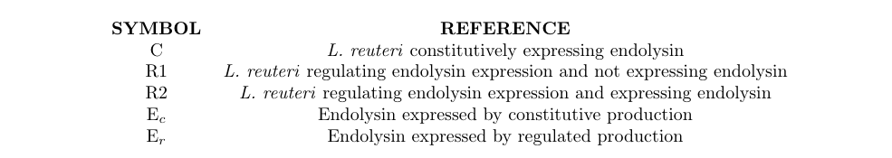
Colour of Graph Line	Explanation
Dotted	L. reuteri constitutively expressing endolysin.
Green	Endolysin yield increases with the time of induction of endolysin expression
Blue	Endolysin yield decreases with the time of induction of endolysin expression
Red	Endolysin yield of note is below endolysin yield from constitutive expression

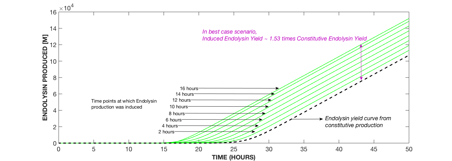
Fig. 1a compares the yield of endolysin from constitutive expression to that from dynamic expression whereby yield increases with increase in the time of induction.

For induction times ranging from 2 hours to 16 hours, the endolysin yield is greater than the endolysin yield from constitutive production.

Additionally, the yield increases with increase in time point at which expression was induced. In the best case scenario, endolysin yield from induced expression at 16 hours is 1.5 times the endolysin yield from constitutive production.

After the 16 hour time point, endolysin yields decrease with increase in the induction time. This is seen in Figure 1b below.

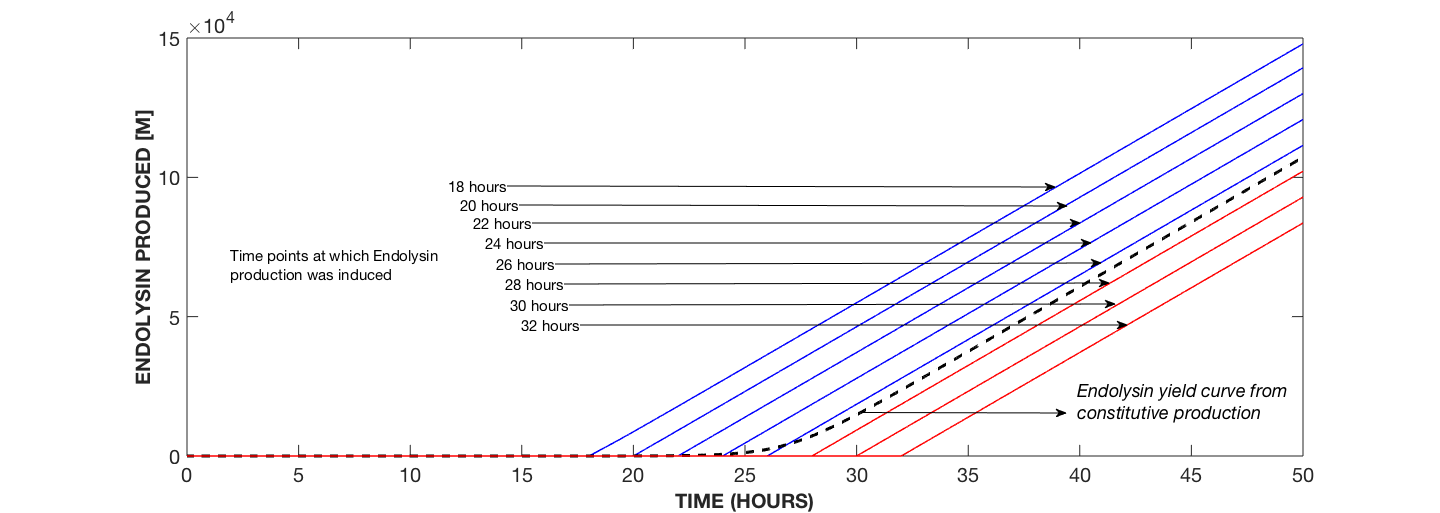
Fig. 1b compares the yield of endolysin from constitutive expression to that from dynamic expression whereby yield decreases with increase in the time of induction.

The graph shows that even though endolysin yields from dynamic expression are higher than those from constitutive expression, the yield decreases when the induction time is increased beyond 16 hours.

After the 28 hour time point, the yield is lower than the yield from constitutive expression and continues to decrease as we increase the induction time.

To analyse the survivability of L. reuteri dynamically expressing endolysin to L. reuteri constitutively expressing endolysin, we plotted the growth curves corresponding to the endolysin yields above. The results are shown in Figure 2 below.

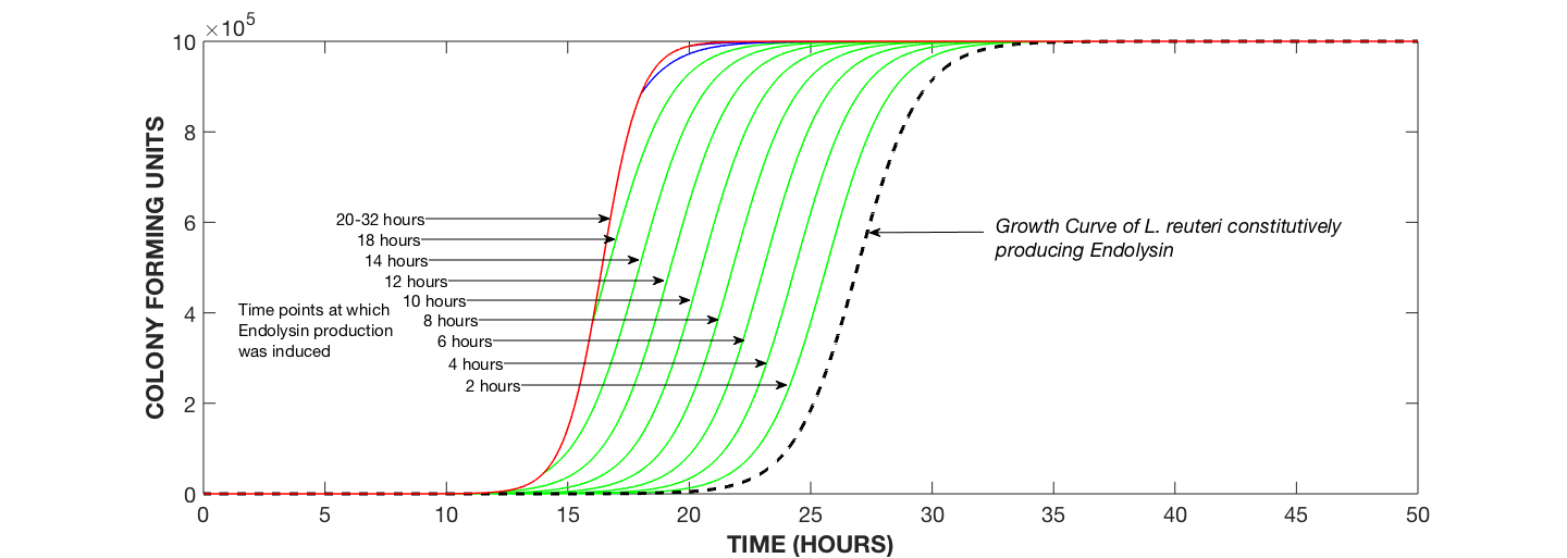
Fig 2: Growth Curves of L. reuteri Undergoing Endolysin Expression with Induction Times ranging from 2 hrs to 32 hrs.

The graph clearly depicts faster growth for L. reuteri undergoing dynamic expression of endolysin. In addition to that, the more endolysin expression is delayed (i.e the greater the induction time), the faster L. reuteri reaches its carrying capacity.

Discussion

From the results above, regulated production has advantages over constitutive production in:

1. Endolysin Yield

If endolysin expression is induced before 18 hours, dynamic endolysin expression results in greater endolysin yields from L. reuteri than constitutive expression.



2. Survivability of L. reuteri

Dynamic endolysin expression reduces cell stress on L. reuteri and substantially increases survivability. This is especially beneficial to our probiotic as it improves the chances of L. reuteri establishing itself in the competitive gut microbiome.

We therefore decided to choose a dynamic expression system, as opposed to a constitutive one, in our probiotic.

Part II: Mathematical Model of Two-Component Regulatory System (TCS)

Once we established that expression of the endolysin in our L. reuteri should be regulated, we needed an external stimulus indicative of C. difficile infection, as well as a regulatory system that would transduce such a stimulus to induce endolysin expression.

External Stimulus Requirements

Given that our aim is to induce expression of endolysin upon detection of pathogenic C. difficile (as opposed to dormant colonies in the gut), the external signal must be a biomarker of the pathogen. Thus, an excellent candidate is the autoinducer peptide (AIP) molecule, a quorum sensing molecule produced by C. difficile to trigger toxin expression in neighbouring C. difficile cells.

Regulatory System Requirements

For optimal function of our overall system, the regulatory system must meet certain requirements:

• Endolysin expression should be triggered when the surrounding population of C. difficile crosses a certain threshold.
• The regulatory system must be robust to temporary spikes of external signal(s).
• Endolysin synthesis should be speedy and produce sufficient amounts of endolysin so that the surrounding population of C. difficile diminishes before toxin synthesis occurs significantly.

After defining the regulatory system requirements above, we then needed to find a suitable regulatory system - either natural or synthetic. As the AIP quorum signalling molecule of C. difficile is relatively uncharacterised, it would be very difficult to engineer a custom receptor. Thus, it made sense to use the two-component AgrA/AgrC regulatory system already in-built into C. difficile.

Thus, we chose to mathematically model this AIP detection and two-component AgrA/AgrC regulatory system to provide a model of our corresponding system in vitro.

Regulatory System Primer

C. difficile uses a two-component system (TCS) to detect its signalling molecule (AIP). As seen below, when the AIP molecule binds to its AgrC receptor, it triggers a phosphorylation cascade: the receptor first autophosphorylates; this causes the phosphorylation of AgrA protein which then dimerises. The dimerised AgrA protein acts as the specific transcription factor for the expression of CD27L endolysin.

Assumptions

1. The modelled environment is uniformly mixed, hence spatial dependencies can be ignored.
2. Dephosphorylation of AgrA protein occurs via housekeeping phosphatases.
3. There is negligible decrease in the concentration of dimerised AgrA protein due to promoter binding as binding of one molecule of dimerised AgrA protein to the promoter is sufficient to trigger endolysin synthesis.
4. Timescale of degradation of all proteins is approximated to be equal as in Jabbari et al. (2009)¹. Consequently, rate of degradation is the same.

Kinetic Equations

Species Key:

Production of AgrAC Proteins:

Transcription

Kinetic Rate Equation	Kinetic Rate Constant	Kinetic Rate Constant Value Modelled
$$[NULL] \to M$$	$$m$$	$$8.33 \ M cell^{-1} \ minute^{-1}$$

Translation + Membrane Insertion of Cytoplasmic AgrC Receptor

Kinetic Rate Equation	Kinetic Rate Constant	Kinetic Rate Constant Value Modelled
$$M \to M + A$$	$$K_a$$	$$8.33 \times 10^{-8} \ minutes^{-1}$$
$$M \to M + C$$	$$K_c$$	$$8.33 \times 10^{-6} \ minutes^{-1}$$
$$C \to R$$	$$\alpha_C$$	$$0.0556 \ minutes^{-1}$$

Binding of AIP Signal to Receptor & Subsequent Signal Transduction

AIP Binding to Transmembrane AgrC Receptor

Kinetic Rate Equation	Kinetic Rate Constant	Kinetic Rate Constant Value Modelled	Inverse Kinetic Rate Constant	Inverse Kinetic Rate Constant Value Modelled
$$S + R \leftrightarrow R_b$$	$$k_{bind}$$	$$1.67 \times 10^{-7} \ (M \times minute)^{-1}$$	$$k_{ibind}$$	$$1.167 \ minutes^{-1}$$

Autophosphorylation of AgrC Receptor

Kinetic Rate Equation	Kinetic Rate Constant	Kinetic Rate Constant Value Modelled	Inverse Kinetic Rate Constant	Inverse Kinetic Rate Constant Value Modelled
$$R_b \leftrightarrow R_{bp}$$	$$k_{autop}$$	$$6.3133 \ minutes^{-1}$$Ref. 3	$$k_{iautop}$$	$$ 10^{-2} \ minute^{-1}$$

Phosphotransfer to AgrA Protein

Kinetic Rate Equation	Kinetic Rate Constant	Kinetic Rate Constant Value Modelled	Inverse Kinetic Rate Constant	Inverse Kinetic Rate Constant Value Modelled
$$R_{b_p} + A \leftrightarrow R_b + A_p$$	$$k_{phosph}$$	$$5 \times 10^5 \ minutes^{-1}$$	$$k_{dphosph}$$	$$0.1777 \ minutes^{-1}$$Ref. 4

Dimerisation of AgrA Protein

Kinetic Rate Equation	Kinetic Rate Constant	Kinetic Rate Constant Value Modelled	Inverse Kinetic Rate Constant	Inverse Kinetic Rate Constant Value Modelled
$$2A_p \leftrightarrow A_{p_2}$$	$$\phi_d$$	$$3.33 \times 10^{8} \ (M \times minute)^{-1}$$	$$\phi_m$$	$$0.0167 \ minute^{-1}$$

Degradation of Molecules

Kinetic Rate Equation	Kinetic Rate Constant	Kinetic Rate Constant Value Modelled
$$X \to NULL \ (where X=M, A, C, R, Rb, Rbp, S, Ap, Ap_2)$$	$$\delta_X$$	$$0.05566 \ minutes^{-1}$$Ref. 2

Differential Equations

Concentration Modelled	Differential Equation	Process Modelled
mRNA of AgrC Receptor & AgrA Protein	$$\frac {dM}{dt} = m - \delta_{M} \times M$$	Transcription of AgrC & AgrA Genes + Degradation of mRNA
Deactivated AgrA Protein	$$\frac {dA}{dt} = K_a \times M - \delta_A \times A - k_{phosph} \times R_{bp} \times A + k_{dphosph} \times R_b \times A_p$$	Translation of AgrA Protein + Degradation of AgrA Protein + Phosphorylation/Dephosphorylation of AgrA
Cytoplasmic AgrC Receptor	$$\frac {dC}{dt} = K_a \times M - \alpha_C \times C - \delta_C \times C$$	Translation of AgrC Receptor + Membrane Insertion of AgrC Receptor + Degradation of AgrC Receptor
Unbound AgrC Receptor	$$\frac {dR}{dt} = \alpha_C \times C - \delta_R \times R + k_{ibind} \times R_b - k_{bind} \times R \times S$$	Membrane Insertion of AgrC Receptor + Degradation of Inserted AgrC Receptor + Binding/Unbinding of AgrC Receptor
Bound AgrC Receptor	$$\frac {dR_b}{dt} = k_{bind} \times S \times R - k_{ibind} \times R_b - \delta_{R_b} \times R_b + k_{iauto} \times R_{bp} - k_{autop} \times R_b + k_{phosph} \times R_{b_p} \times A - k_{dphosph} \times R_b \times A_p$$	Ligand Binding/Unbinding of AgrC Receptor + Degradation of Bound AgrC Receptor + Autophosphorylation/De-autophosphorylation + Phosphotransfer/Dephosphorylation of AgrC Receptor
Phosphorylated AgrC Receptor	$$\frac {dR_{b_p}}{dt} = k_{autop} \times R_b - k_{iauto} \times R_{b_p} - k_{phosph} \times R_{b_p} \times A + k_{dphosph} \times R_b \times A_p - \delta_{Rb_p} \times R_{b_p}$$	Autophoshorylation/Auto-dephosphorylation of AgrC Receptor + Phosphotransfer/Dephosphorylation to AgrA Protein + Degradation of Phosphorylated AgrC Receptor
AgrA Protein	$$\frac {dA_p}{dt} = k_{phosph} \times R_{bp} \times A - k_{dphosph} \times R_b \times A_p - 2 \times \phi_d \times A_{p}^2 + \phi_m \times A_{p_2} - \delta_{A_p} \times A_p$$	Phosphotransfer/Dephosphorylation of AgrA Protein + Dimerisation/Monomerisation + Degradation of AgrA Protein
Dimerised AgrA Protein	$$\frac {dA_{p_2}}{dt} = \phi_d \times A_{p}^2 - 0.5 \times \phi_m \times A_{p_2} - \delta_{Ap_2} \times A_{p_2}$$	Dimerisation/Monomerisation of AgrA Protein + Degradation of Dimerised AgrA Protein

Upregulation of Cells

Guided by the mathematical model built by Jabbari et al. (2009)², we constructed a differential equation to track the upregulation state of each cell based on the binding kinetics of the transcription factor. This is further elaborated below.

Consider the parameter P that measures the fraction of bacterial population that is upregulated at any given time (P = 1 if the entire population is upregulated, and P = 0 if the entire population is downregulated).

In Jabbari et al. (2009)², the following differential equation described the upregulation of S. aureus cells:

$$\frac {dP}{dt} = b \times \frac {A_p}{N} \times (1-P) - u \times P$$

The particular parameters are explained in the table below.

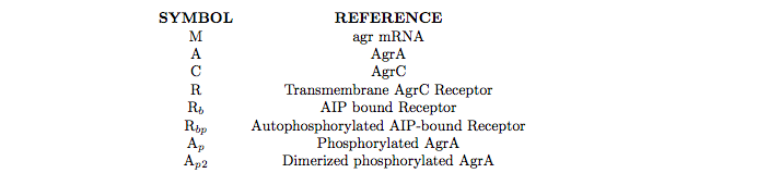
Parameter	Explanation
b	Binding Rate of Transcription Factor
u	Unbinding Rate of Transcription Factor
Ap	Population-wide Concentration of Transcription Factor in the S. aureus Quorum Sensing System
N	Number of Cells

In the above differential equation, $$b \times \frac {A_p}{N} \times (1-P)$$ describes the increase in the fraction of upregulated cells due to the binding of the transcription factor to the promoter, and $$u \times P$$ accounts for the decrease in fraction of upregulated cells due to the unbinding of transcription factor from the promoter.

In our particular ProQuorum system, the transcription factor is the dimerised phosphorylated AgrA protein. Thus, for our particular system, the different equation amounts to:

$$\frac {dP}{dt} = b \times \frac {A_{p_2}}{N} \times (1-P) - u \times P$$

The above differential equation describes the upregulation state of the population on a gradient from 0 to 1 based on the binding kinetics of the transcription factor to the promoter.

As we are only considering dynamics in a single cell, we set N=1 to obtain:

$$\frac {dP}{dt} = b \times A_{p_2} \times (1-P) - u \times P$$

The above equation maps the upregulation state of a single cell on a gradient of 0 to 1. However, in reality a single cell can either be upregulated to produce endolysin or not be upregulated. Therefore, we need to approximate the upregulation state to an integral value of 0 or 1.

To perform such an approximation, we introduce the concept of an upregulation cut-off. The upregulation cut-off refers to the threshold value of P over which a cell will become upregulated and express endolysin. Here, we have taken the upregulation cut-off to be 0.75, or 75 %.

Results

To analyse the key features of the two-component regulatory system within each cell, we ran cellular-scale simulations in which the cell is exposed to various signal concentrations and patterns.

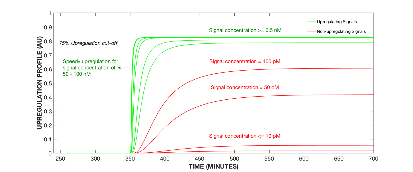
Figure 1. Upregulation Profile for Varying AIP Concentrations

As depicted in Figure 1 above, AIP concentrations below the concentration of 0.5 nM are unable to reach the 75% upregulation cut-off, and consequently fail to upregulate the cell.

Additionally, for AIP concentrations equal to or greater than 0.5 nM, the time taken to reach the upregulation cut-off decreases with increasing AIP concentration, implying that stronger signals take less time to upregulate the cell.

To observe how the concentration of the transcription factor varies during upregulation and downregulation, we ran a simulation where an AIP concentration of 1nM was inserted at 350 hours and taken away at 650 hours.

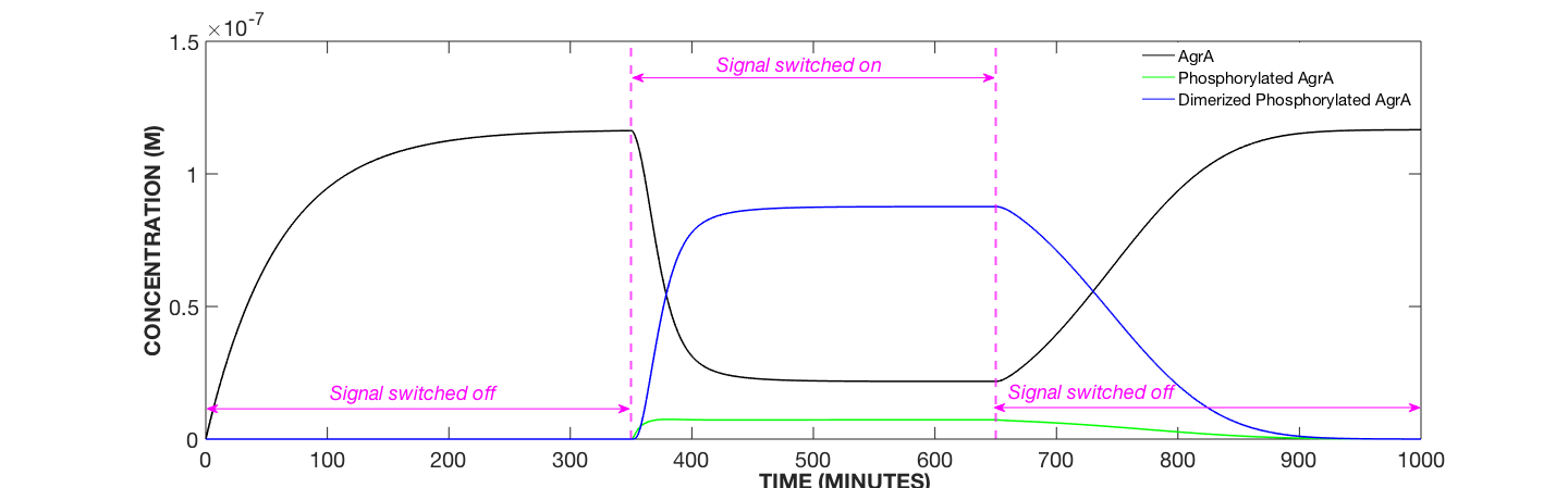
Figure 2. Transcription Factor Dynamics, AIP Concentration Modulated

As observed in Figure 2 above, the time taken by dimerized phosphorylated AgrA to reach its steady state during upregulation is less than the time taken to reach its steady state during downregulation.

The dynamics of AgrA caused by the modulation of AIP concentration is reflected in the upregulation profile of the cell as depicted in Figure 3 below.

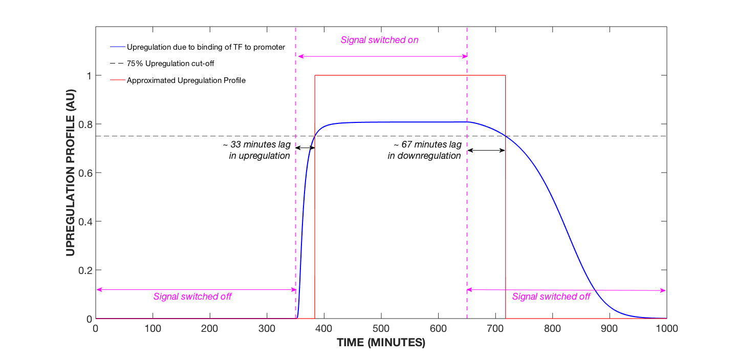
Figure 3. Upregulation Profile of Cell, AIP Concentration Modulated

Furthermore, the delay in upregulation of the cell after the AIP signal has been turned on is approximately 33 minutes. Thus, if the duration of active AIP signalling is less than approximately this time, the cell would ultimately not upregulate.

For further insight into the delay in upregulation of the cell, we plotted the maximum upregulation state of the cell for different signal durations given 1 nM AIP signal concentrations.

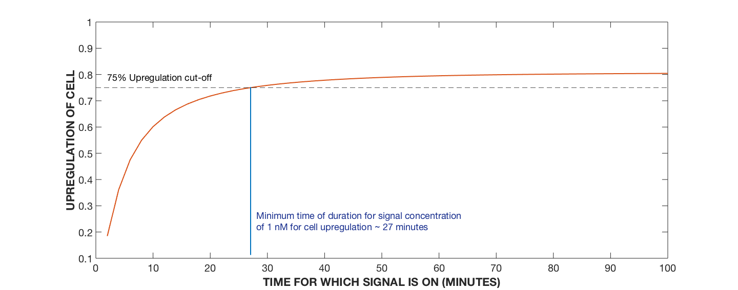
Figure 4. Upregulation Profile of Cell, Varying AIP Signalling Time

Figure 4 above illustrates how the cell fails to upregulate for signal durations below 27 minutes, as previously estimated in FIgure 3.

When running the same simulation for different signal concentrations, we obtain the following graph:

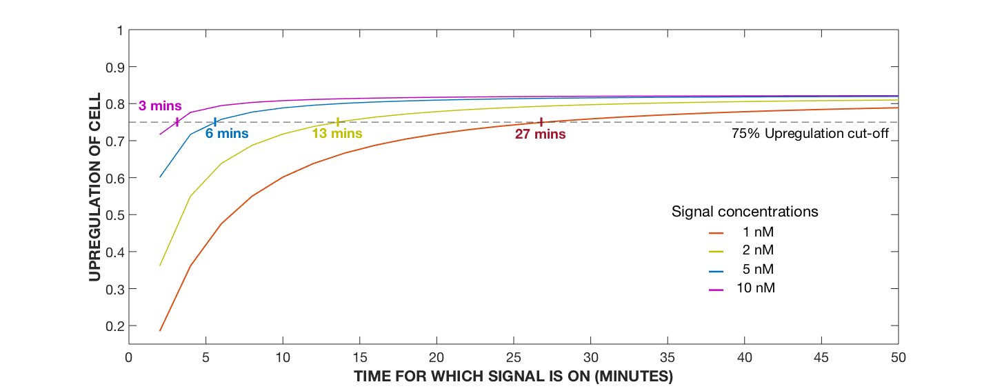
Figure 5. Upregulation Profile of Cell, Varying AIP Signalling Time with Varying AIP Concentrations

Figure 5 above indicates that the minimum signal time duration for upregulation decreases with increasing signal concentrations. This is ideal because given that higher concentrations of AIP correspond to larger C. difficile colonies, it is beneficial for our system to react faster than for lower signal concentrations.

For the mathematical model built so far, the minimum signal concentration required for upregulation is 0.5 nM. However, one of our design requirements was that the probiotic must begin endolysin synthesis before significant toxin synthesis has occurred. To meet this design requirement, each cell of L. reuteri must be sensitive to picomolar quantities of AIP.

To make L. reuteri more sensitive to the AIP signal, we could engineer the cells to produce more receptor proteins.

Thus, we changed the kinetic constant Kc in the mathematical model from $$8.33 \times 10^{-6}$$ per minute per mRNA copy to $$8.33 \times 10^{-4}$$ per minute per mRNA copy and ran simulations to test the minimum signal concentration required to upregulate the cell.

As seen in Figure 6 below, the cell was ultimately upregulated by AIP signal concentrations in the picomolar range:

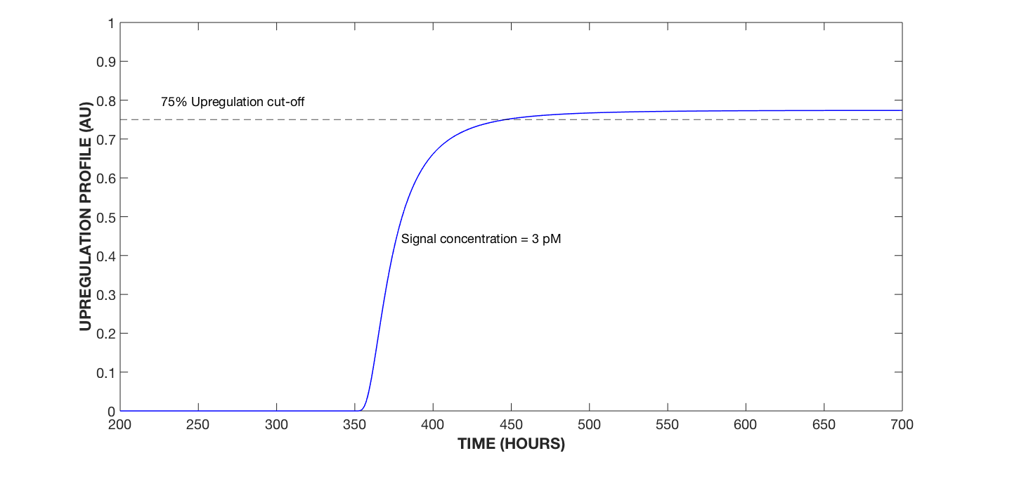
Figure 6. Upregulation Profile of Cell, 3 pM AIP Signal Concentration

Discussion

The two-component regulatory system employed by C. difficile has been confirmed via our model to meet the following design requirements:

• Endolysin expression is triggered only after the concentration of AIP crosses a certain threshold - a valid indicator of C. difficile population density.
• Endolysin expression is robust to sudden and short-lived spikes in AIP concentration due to its intrinsic delay in response.

After analyzing the two component regulatory system to be used in our probiotic, we developed our cellular mathematical model into a population wide mathematical model to analyse how our probiotic would cope against a growing C. difficile infection. This is further detailed in our Therapeutic Insight page.

References

#	Reference
1	Jabbari, Sara, et al. “Mathematical Modelling of the Agr Operon in Staphylococcus Aureus.” Journal of Mathematical Biology, vol. 61, no. 1, 2009, pp. 17–54., doi:10.1007/s00285-009-0291-6.
2	Wright, J. S., et al. “Transient Interference with Staphylococcal Quorum Sensing Blocks Abscess Formation.” Proceedings of the National Academy of Sciences, vol. 102, no. 5, 2005, pp. 1691–1696., doi:10.1073/pnas.0407661102.
3	Srivastava, S. K., et al. “Influence of the AgrC-AgrA Complex on the Response Time of Staphylococcus Aureus Quorum Sensing.” Journal of Bacteriology, vol. 196, no. 15, 2014, pp. 2876–2888., doi:10.1128/jb.01530-14.
4	Wang, Boyuan, and Tom W. Muir. “Regulation of Virulence in Staphylococcus Aureus : Molecular Mechanisms and Remaining Puzzles.” Cell Chemical Biology, vol. 23, no. 2, 2016, pp. 214–224., doi:10.1016/j.chembiol.2016.01.004.