MODELING

SCU-China Header

COMPUTIONAL STRUCTURAL BIOLOGY

a

Introduction

In the metabolic circuit of cordycepin and pentostatin, the three key enzymes called Cns1, Cns2 and Cns3 are first discovered in 2017 (Xia Y et al., 2017), and they are poorly studied, with no structures published, which makes our project a black box without knowing the catalytic mechanism and blocks the further development of enzyme engineering conducting on them. Based on this situation, we constructed structural prediction, molecular dynamic simulation to enrich the characterization of the structural properties of the enzymes step by step. Additionally, we use molecular dynamic simulation and molecular docking to help determine which linker of the fusion expression proteins is prior to choosing for experiments.

Structure Prediction

Having only the sequences of the enzyme Cns1, Cns2, and Cns3, the first thing to do is to build the three-dimensional structures of the enzymes. With no access to either of the methods for protein structural analysis, including Nuclear magnetic resonance (NMR), x-ray crystallography and cryo-electron microscopy (Cryo-EM), we turned to the use of structure prediction.

Homology Modeling

Protein structure prediction is a mapping from the amino acid sequence of a protein to the three-dimensional structure. It is highly important in medicine and biotechnology although it is not as accurate as the structure from the experiments. It is observed that similar sequences often adopt similar protein structures, which form the foundation of homology modeling.

As the most popular type of protein structure simulation method, we constructed homology modeling based on servers and softwares including SWISS-MODEL (Waterhouse et al., 2018) and Modeller (Webb B et al., 2014).

Using SWISS-MODEL, we found that the template coverage of Cns1, Cns2 and Cns3 is 41%, 76%, and 26%. The result of homology modeling is accurate when the template coverage if above 60%, and is not reliable when the template coverage below 30%.

protein	coverage	assessment of coverage
cns1	41%	fairly reliable
cns2	76%	reliable
cns3	26%	not reliable

Considering Cns3 protein, we use Modeller to try again. The template searching process failed with the threshold E-value of 10, which is the bottom line of the protein sequences. The result shows that Modeller can not find the aligned template in protein structure database which is in the range of the threshold.

Evaluating the model of Cns2 reveals the low GMQE (0.50) and QMEAN Z-score(<-5.9), which indicate the low quality of the result model. Likewise, the low GMQE (0.23) and QMEAN Z-score (<-6.1) indicate that the result is bad.

GMQE (Global Model Quality Estimation) is a quality estimation which combines properties from the target–template alignment and the template search method. The resulting GMQE score is expressed as a number between 0 and 1. Higher numbers indicate higher reliability.

The QMEAN Z-score indicates whether the QMEAN score of the model is comparable to what one would expect from experimental structures of similar size. QMEAN Z-scores around zero indicate good agreement between the model structure and experimental structures of similar size. Scores of -4.0 or below are an indication of models with low quality.

In conclusion, our attempt of using homology modeling to get the structure information of the enzymes failed as the low quality of the result. We will try other methods to predict the structure of the other two proteins.

Fold Recognition

Being blocked by the bad strcuture prediction result of Cns1 and Cns3, we consult Prof. Cao Yang for other methods of structure prediction. He recommended a server called ITASSER (Yang J et al., 2014) which is a powerful structure prediction tool based on fold recognition. More details about our consultation with Prof. Cao.

Fold recognition is another method of protein modeling. It differs from the homology modeling method of structure prediction as it is used for proteins which do not have their homologous protein structures deposited in PDB, whereas homology modeling is used for those proteins which do. From its definition, we know that it solves our problem quite well, because we can not find any fair template for Cns1 and Cns3.

The result of the prediction by ITASSER is as follows:

protein	C-score
cns1	-3.74
cns2	0.70
cns3	-1.10

The confidence of each model is quantitatively measured by C-score is typically in the range of [-5, 2], where a C-score of a higher value signifies a model with a higher confidence and vice-versa.

The resulting C-score of Cns1 reveals that the prediction is not good, with fair result of Cns3 and good result of Cns2. From the predicted structure, we can find that the His tags of all the three enzymes are away from the catalytic cores, thus not affecting the catalytic activities.

Comparing the predicted structure of Cns1 by SWISS-MODEL and ITASSER, we found some interesting common points.

Figure. 1 Structure predictions of Cns1 protein from SWISS-MODEL and ITASSER. The red one is the structure from SWISS-MODEL, only covering the template sequence, and the cycan one is the structure from ITASSER.

The structure from SWISS-MODEL only recognises a proportion of the whole sequence of Cns1, which froms a homo-tetramer. Alignment between the monomer and the structure from ITASSER is illutrated in figure. The result shows that the result from ITASSER gives more information although this part of information is not accurate (the structure in blue, aside from the alignment area, is unreliable). The two structures from both softwares have high similarities at the alignment area, which indicates that this area is more reliable.

Analysis of ligand binding sites by ITASSER reveals that it is located in this alignment area, which suggests that the inaccuracy of the other parts does not affect its functional characterisation.

Figure. 2 Activity core of Cns1 protein predicted by ITASSER, drawn in red. Other residues are drawn in green.

When we turned to the result of Cns2 prediction, we aligned the predicted structure by ITASSER with that by SWISS-MODEL and found that the RMSD between the two is 1.492nm (aligned by Pymol), which indicates that they are quite similar.

Figure. 3 Structure comparison of Cns2 protein predicted by SWISS-MODEL and ITASSER. The green one is the result by SWISS-MODEL while the cyan one is by ITASSER.

Likewise, when we analysed the ligand binding sites of the predicted structures by SWISS-MODEL and ITASSER, when found that they are at the same position although the depth of the catalytic pocket is different. This phenomenon gived a strong support to our validity of structure prediction, which did enrich the characterisation of the structural properties of the enzymes.

Figure. 4 Elucidation of the activity core of Cns2 protein. Left is the structure predicted by ITASSER (cycan), in which the activity core is drawn in red. Right is the structure alignment between predicted results from ITASSER (cycan) and SWISS-MODEL (green). Likewise, activity core is drawn in red.

Considering Cns3, the result is not acceptable, especially the structure of the HisG domain (in orange). A $\alpha$ helix of HisG domain stretches out abruptly, which is not natural in protein. However, from the predicted result of Cns3, we can attain some information. A bunch of $\alpha$ helixes lay parallelly at the core of the protein, forming a kind of structural scaffold that supports the structural stability of NK and HisG domain. The functional domains of Cns3 lay independently outside of the core. Therefore, from the angle of structural biology, in theory, separation of the two domains will not affect the individual function of each domain as they work separately. This conclusion had a theoretical guideline for the separate use of HisG domain of Cns3 in our experimental design.

Figure. 5 Predicted structure of Cns3 protein by ITASSER. NK domain is drawn in cyan, NK domain is drawn in orange and other residues are drawn in green.

Owing to some inappropriate factors in the prediction, we further use molecular dynamic simulation to adjust the structure.

Molecular Dynamic Simulation

The prediction of the enzyme structures gave us amounts of useful information. However, it exists some improper structure in some part of the result. In order to adjust the inappropriate structure from the structure prediction process and investigate the ligand-enzyme interaction using molecular dynamics (MD).

In our project, we use GROMACS, which is one of the most popular MD software packages for protein, lipid, and nucleic acid. The version of GROMACS we used is 5.0.7, which is run on Linux server provided by Prof. Cao. More details about the help from Prof. Cao.

Adjustment of the predicted structure

Molecular dynamics allows us to assess stability of the predicted structure of our enzymes and obtain new models that are more likely to be the native conformation in solvent which would be the possible state in our wet lab and the factory.

Steps of the utility of GROMACS are derived from the GROMACS tutorial and are summarised to SCU-China 2019 GROMACS protocol which in some details is slightly different from the tutorial.

Briefly, we generated the topology of the enzyme structure, and put it in a box (the figure below), in which we filled in water and ions. We conducted energy minimization using the gradient descent method. After the energy minimization, we performed a position-restricted pre-equalization simulation and conducted the final simulation. After some time, we can get the trace file of the simulation which can be transformed into figures.

Figure. 6 Simulation box, which is filled with protein, water molecues and ions. Simulation process is conducted in this box. Users should ensure the protein in the box.

According to the GROMCAS tutorial, the final simulation after equilibrium is 1ns in totoal. Therefore, we firsly conducted the simulation for 1 nanosecond. The results for the three enzymes are as follows:

Figure. 7 Molecular dynamic traces of Cns1, Cns2 and Cns3 in solution, simulated for 1 nanosecond. GROMACS version: 5.0.7, run on Linux server.

For each enzyme, the corresponding parameters including the potential energy fluctuation and temperature fluctuation are depicted below:

Figure. 8 Elucidation of potential energy fluctuation and temperature fluctuation of Cns1, Cns2 and Cns3 simulation for 1 nanosecond. The top two pictures are the results of Cns1, in the middle are the results of Cns2, and the bottom are the results of Cns3.

We can draw a conclusion from the results above that the structures of Cns1, Cns2 and Cns3 are getting more stable and the average temperature in which the structures are stable is around 300K.

Alignment between the initial structures and the simulated structures will give us a straight overview of the simulation process.

Figure. 9 Alignment between initial structure and simulated structure simulated for 1 nanosecond. From top to bottom are alignments of Cns1, Cns2, and Cns3. Initial structures are drawn in blue and simulated structures are drawn in red. Alignment and pictures are generated by Pymol.

Alignment of Cns1 initial structure and its simulated structure shows that it changes little in the head, which is the enzyme catalytic site while it changes a lot in its long tail. This result supports that the structure of the tail is not reliable while the head is reliable. Likewise, the analysis of Cns2 reveals that this structure is reliable and the enzyme catalytic site is in its center. Interestingly, the result of Cns3 shows that the structure of HisG domain changes a lot and has a tendency of curling up and folding.

Further investigation of the alignment of Cns2 initial structure and its simulated structure in surface mode reveals that the core is not destroyed during molecular kinetic simulation and the catalytic pocket is shallower than the initial structure.

Figure. 10 Alignment between initial structure and simulated structure of Cns2 protein shown in surface. Initial structure is drawn in blue and simulated structure is drawn in red.

The backbone RMSD between the initial structure and the simulated structure is plotted below:

Figure. 11 Elucidation of backbone RMSD between initial structures and simulated structures of Cns1, Cns2, and Cns3 protein. Simulated time is 1 nanosecond.

The RMSD plot above shows a fatal error in the simulation result. Overall, the RMSD lines are constantly rising with some fluctuation, which means that the result of simulation is not the final state of the MD simulation. If we extend the time of the simulation, probably, to 10ns, the final conformation would like to change to another state, a more stable and low-energy state.

Considering the problem above, we changed our protocol which is originally derived from the GROMACS tutorial and extend the time to 10ns. The result is more reliable actually, but costs much more time in return.

The 10-nanosecond simulations are shown below:

Figure. 12 Molecular dynamic traces of Cns1, Cns2 and Cns3 in solution, simulated for 10 nanoseconds. GROMACS version: 5.0.7, run on Linux server.

For each enzyme, the corresponding parameters including the potential energy fluctuation are depicted below:

Figure. 13 Elucidation of potential energy fluctuation and temperature fluctuation of Cns1, Cns2 and Cns3 simulation for 10 nanoseconds. The top two pictures are the results of Cns1, in the middle are the results of Cns2, and the bottom are the results of Cns3.

Alignment between the initial structures and the 10-nanosecond simulated structures is shown below.

Figure. 14 Alignment between initial structure and simulated structure simulated for 10 nanoseconds. From top to bottom are alignments of cns1, cns2, and cns3. Initial structures are drawn in blue and simulated structures are drawn in red. Alignment and pictures are generated by Pymol.

The backbone RMSD is plotted below, RMSD of cns2 and cns3 protein reaches a convergence after 10-nanosecond simulation but RMSD of cns1 does not. It seems that the simulated structure of cns1 is not the stable structure and will adjust further if time permitted. From the tendency of the structure, we can see that the red arm stretching out of the core will gradually fold and adjoin to the activity core based on the result of 10-nanosecond simulated stricture.

Figure. 15 Elucidation of backbone RMSD between initial structures and simulated structures of Cns1, Cns2, and Cns3 protein. Simulated time is 10 nanoseconds.

Since HisG is a relatively independent domain in Cns3 enzyme and it is reported in Cordyceps militaris that HisG produces pentostatin independently, it should be valid that the structure of HisG alone remains its catalytic activity. Therefore, we would like to investigate further on the structure of HisG domain.

We performed structure prediction by ITASSER and molecular docking by SWISS-Dock for HisG. The result is below:

Figure. 16 Elucidation of molecular docking between the predicted structure of HisG and adenosine. The picture shows all docking possibilities.

The small molecules are the potential binding conformation of adenosine, which is the substrate. It shows some probable binding sites of adenosine to HisG domain. However, this structure is not natural from the angle of structural biology because it has two huge pockets which are much bigger than they should be. Therefore, we conducted molecular dynamics simulation further for this structure of HisG. The 10-nanosecond simulation is below:

Figure. 17 Molecular dynamic simulation of HisG in solution for 10 nanoseconds. GROMACS version: 5.0.7, run on Linux server.

The simulated structure of HisG domain of Cns3 protein shows a smaller and deeper package in catalytic core compared with the initial predicted structure.

Figure. 18 Alignment between initial structure and simulated structure of HisG simulated for 10 nanoseconds. The initial structure is drawn in blue and simulated structure is drawn in red.

Apart from enabling a more reliable structure in solution, molecular dynamic simulation can set up a simulation system containing a protein in complex with its ligand. Here in our project, we simulated the complex of HisG protein and its ligand adenosine. We altered the typical manual and build our own more suitable in our case. Protocol of protein-ligand molecular dynamic simulation.

We simulated the process of the ligand approaching to the protein and finally binding to the activity core.

Figure. 19 Left is molecular dynamic simulation of the complex formed between HisG and adenosine. Simulation is initialized given the independent structure of HisG and adenosine. At the end of the simulation, adenosine approaches and binds to the package at N-terminus. Right is additional 1 nanosecond simulation of the complex after 10 nanoseconds simulation.

From this simulation, we confirmed the affinity between HisG and adenosine and found out the interaction site, which is the potential activity core. The structure and affinity prediction convinced us that HisG would work well in Saccharomyces cerevisiae. More details about the function validation of HisG domain by experiment.

Linker Determination

The designing principle and evaluation of the linker between two proteins used in fusion expression are obscure, so it is challenging to design linker from scratch. Although some linkers can be found in some articles, but we have no idea if these linkers fit our project well unless doing experiments. However, the painstaking vector construction and function tests prevent us from doing so. Therefore, we would like to use comprehensive bioinformatic methods to evaluate the linkers collected from articles from the structural biological angle.

Linker is used to connect two proteins without destroying respective enzymatic activities. Appropriate linker can minimize the interruption between proteins. In our linker determination model, we would like to predict the structures of fusion protein using different linkers typically utilized in other articles. Comparing those predicted structures, we have to determine the best linker which in maximum prevents interaction between proteins.

Linker search and analysis

We have collected five linkers potential to use:

Flexible linker

GGGGSGGGGSGGGGS

GGGGGGGG

Rigid Linker

EAAAKEAAAKEAAAK

SEAAAREAAAREAAAREAAAR

AEAAAKEAAAKEAAAKEAAAKALEAEAAAKEAAAKEAAAKEAAAKA

We connected Cns1 and Cns2 by these linkers and generated five sequences that are delivered to the ITASSER server and got predicted structures.

From the predicted and simulated structure of Cns1, the activity core is in the range of 443-570, so we evaluated the area in this range if it was unbroken. We chose the best linker which in maximum kept the area intact.

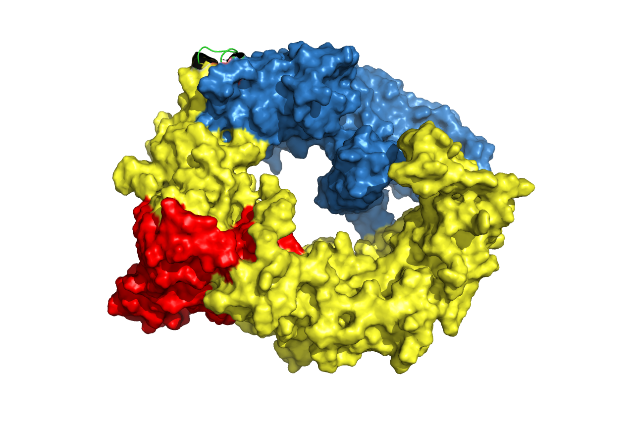
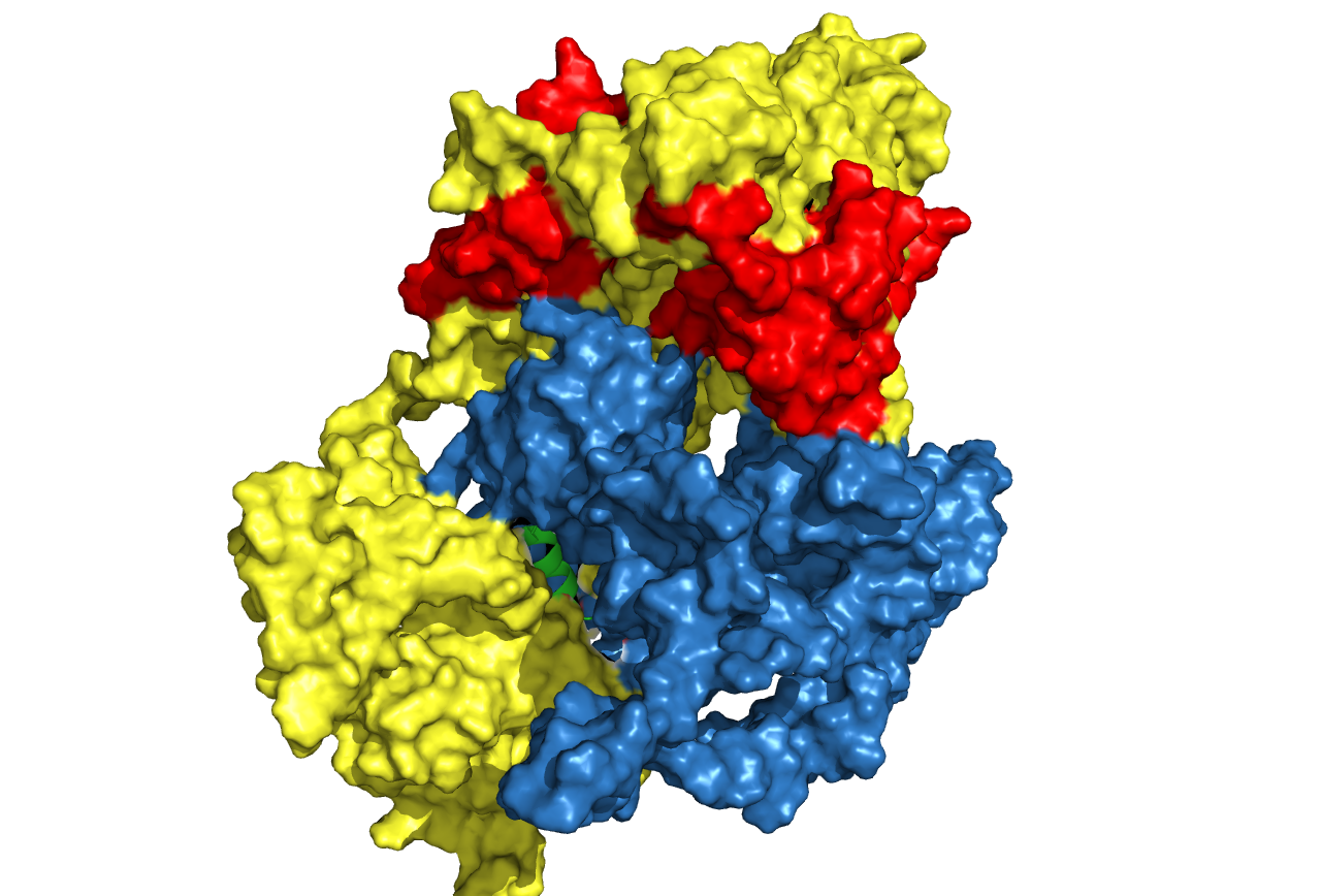
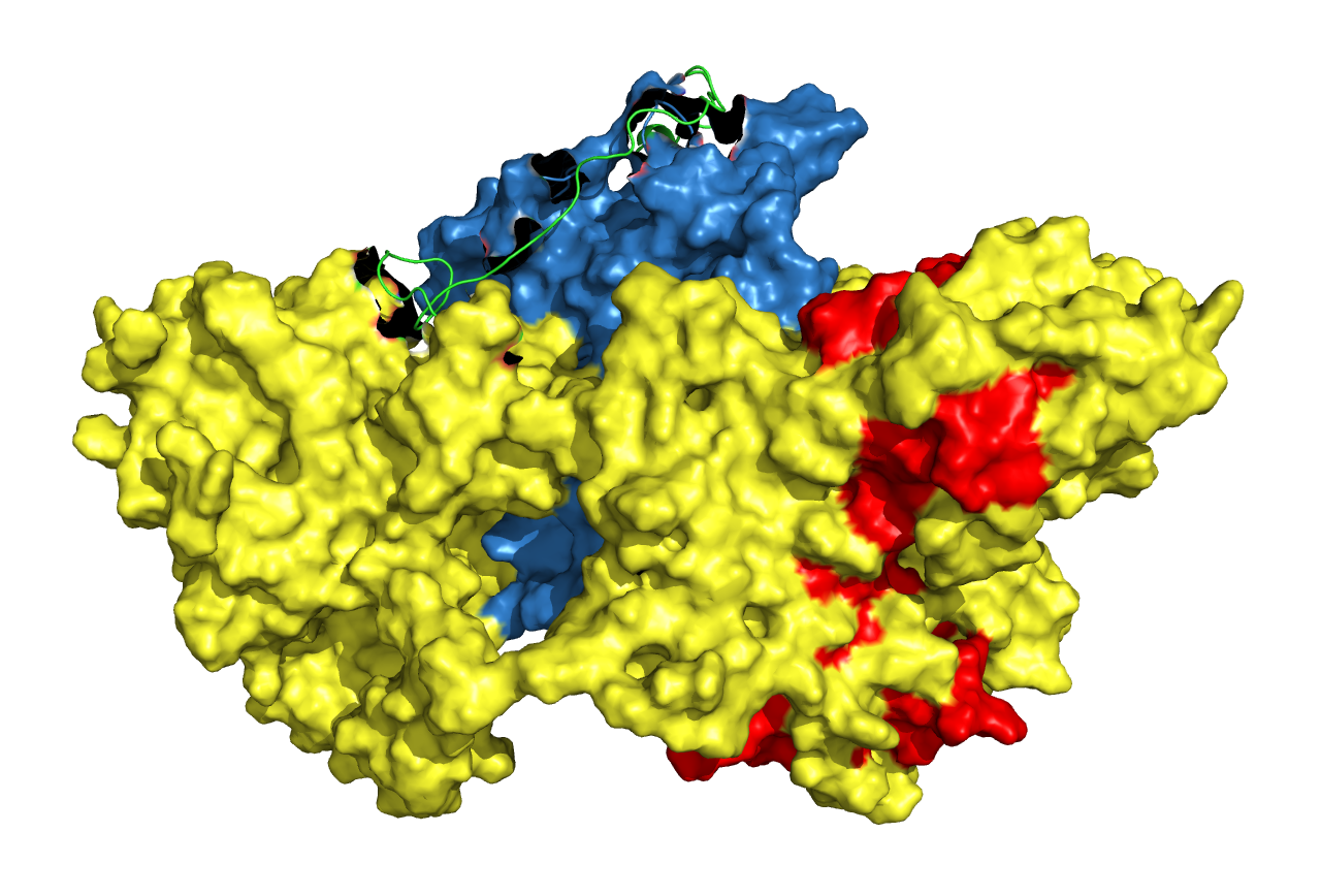
Figure. 20 Structure prediction of cns1-linker-cns2 fusion protein. Linkers are chosen according to research articles (in the table above). Cns1 domain is drawn in yellow while its activity domain is drawn in red and Cns2 is drawn in blue. From left to right, from top to bottom, the linkers are (GGGGS)3, (G)8, (EAAAK)3, S(EAAAR)4 and A(EAAAK)4ALEA(EAAAK)4A respectively.

Analysis from the predicted structures gave us a guideline for choosing the best linker. Cns1 activity domains (areas in red) of the first, third and fifth structures above are dispersed by the disturbance from Cns2 while the other two structures are not. This result revealed that (G)8 and S(EAAAR)4 linker is better than others. Comparing the two linkers, (G)8 is a flexible linker and it enables a closer distance between Cns1 and Cns2 while S(EAAAR)4 is a rigid linker. Alpha-helix formed by S(EAAAR)4 linker works better on dispersing two proteins. Based on all analyses derived above, we chose S(EAAAR)4 for our experiment.

Modeling session provided an optional linker for experiments and Cns1A2_S(EAAAR)4 protein was constructed in experiments. More details about Cns1A2 construction and expression

cns1-linker-cns2? cns2-linker-cns1!

When we designed the fusion protein of Cns1 and Cns2, we determined the linker by comprehensive computational biological methods and connected these two proteins by this linker. We constructed Cns1-linker-Cns2 by default in experiments.

Plasmid construction of Cns1-linker-Cns2 has been constructed and transformed into yeast cells. However, function validation of Cns1-linker-Cns2 shew little cordycepin detected by HPLC. More details about Cns1-linker-Cns2 function validation. The result from the HPLC experiment reveals the weak catalytic activity.

When we reviewed our whole project, we found the potential mistake resulting in weak Cns1-linker-Cns2 activity. In our structure prediction section, we found that the activation domain is at its C-terminus. When we connected the two proteins in the order of Cns1, linker, and Cns2, the activity domain was likely to be disturbed because it was too close to the linker although best linker was chosen.

Based on the hypothesis, we simulated the structure of Cns2-linker-Cns1 to see if it was better to connect the C-terminus of Cns2 to the N-terminus of the linker. Likewise, we used ITASSER to predict the structures. Prediction results are shown below:

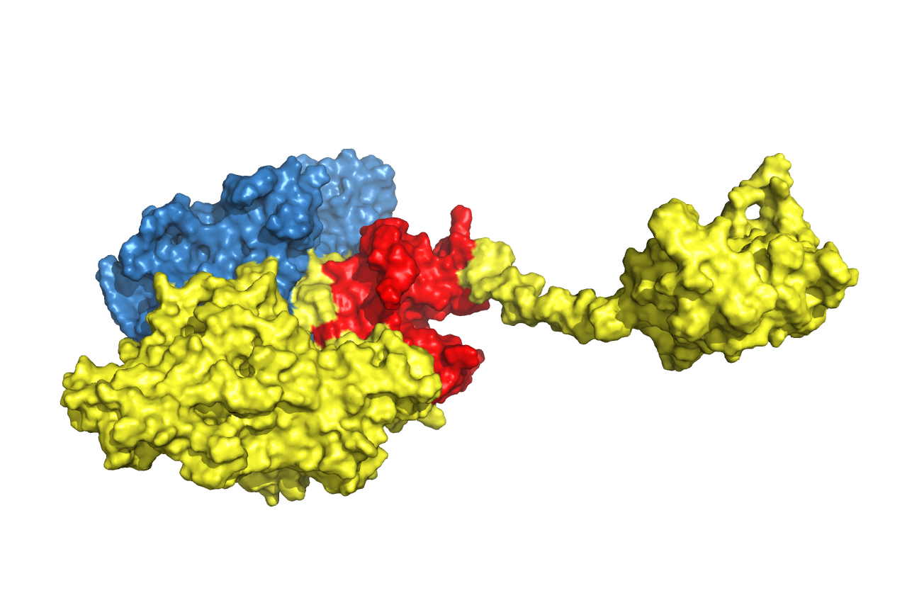
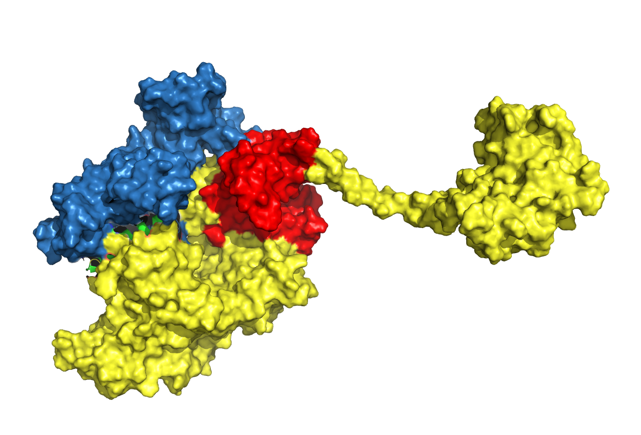
Figure 21. Structure prediction of Cns2-linker-Cns1 fusion protein. Linkers are chosen according to research articles (in the table above). Cns1 domain is drawn in yellow while its activity domain is drawn in red and Cns2 is drawn in blue. From left to right, from top to bottom, the linkers are (GGGGS)3, (EAAAK)3, S(EAAAR)4 and A(EAAAK)4ALEA(EAAAK)4A respectively.

From the result above, we came to a conclusion that connecting the proteins in the order of Cns2, linker, and Cns1 was better than the reverse order. Structural features of activity domains in the first three pictures are similar, while the activity domain of the last one is situated at another side.

In conclusion, Cns1-linker-Cns2 is probably of low activity because of structural disturbance while Cns2-linker-Cns1 provides an intact structure of activity domain. This is the potential reason for little cordycepin detected by HPLC. In future work, we would like to reconstruct the fusion protein Cns2-linker-Cns1 in experiments and perform corresponding function verification.

Reference

Xia, Y. , Luo, F. , Shang, Y. , Chen, P. , Lu, Y. , & Wang, C. . (2017). Fungal cordycepin biosynthesis is coupled with the production of the safeguard molecule pentostatin. Cell Chemical Biology, S2451945617303276.

Waterhouse, A., Bertoni, M., Bienert, S., Studer, G., Tauriello, G., Gumienny, R., Heer, F.T., de Beer, T.A.P., Rempfer, C., Bordoli, L., Lepore, R., Schwede, T. (2018). SWISS-MODEL: homology modelling of protein structures and complexes. Nucleic Acids Res. 46(W1), W296-W303.

Webb, B. , & Sali, A. . (2014). Comparative protein structure modeling using modeller. Current Protocols in Bioinformatics, 47.

Yang, J. , Yan, R. , Roy, A. , Xu, D. , Poisson, J. , & Zhang, Y. . (2014). The i-tasser suite: protein structure and function prediction. Nature Methods, 12(1), 7-8.

Team:SCU-China/ComstrBio