Team:Marburg/Model
Growth Curves
Synthetic Biology was created by introducing engineering principles into the previously existing discipline of biology.
While this came with numerous advantages, one of the most important was the standardization and characterization of parts that larger biological system are built of.
Only with this toolbox of modular, well characterized parts the current achievements in companys like gingko bioworks or the teams of the iGEM competition were made possible and the biobrick standard is a great example.
Not only does this process allow for standardized parts, it also allows to critically question generally agreed on methodologies that otherwise might negatively influence either the reproducibility or performance of experiments.
However, this standardization is not fully a past achievement but an ongoing process.
We noticed during the research how to optimally grow our cyanobacteria that this process still needs alot of standardization.
This was when we decided that we want to critically question all things currently state of the art and this developed into a project in which we used expertise acquired in chemistry, physics, mathematics and biology in addition to sythetic biology.
For example, in the literature the optical density of a culture is sometimes measured with the absorption at 730 nm [Ungerer et al 2018] and sometimes at 750 nm [Russo et al 2019].
Since many labs do not have a spectrometer that is able to measure absorption at 750 nm, we decided after valuable input from James Goldento measure OD at 730 nm.
Light intensity measurements
One of the first aspects that we found to be unsufficiently or contradictorily documented was the light intensity the cultures need to grow optimally.
Also, the state of the art measururement for light intensity used when describing growth of cyanobacteria is Einstein, which is a non SI unit.
Einstein describes the number of photons that arrive in one second at an area of one square metre, one Einstein being one mole (6.022*10**23) of photons /m2 *s.
Most of the times when this unit is used in combination with photosyntetic organisms, not all photons are counted but only photosinthetically active photons with a wavelength betwenn 400 and 700 nanometers.
Since Einstein is not an SI unit, there are no clear definitions how to use it which opens up possibilities for introducing errors.
Due to this for example the definition of photosynthetic photons could be a point that differs between different research groups and is not specifically defined in most publications.
To investigate if there is a better unit to use and if so what and how it should be used, we did an analysis of light units that we describe in the following foray:

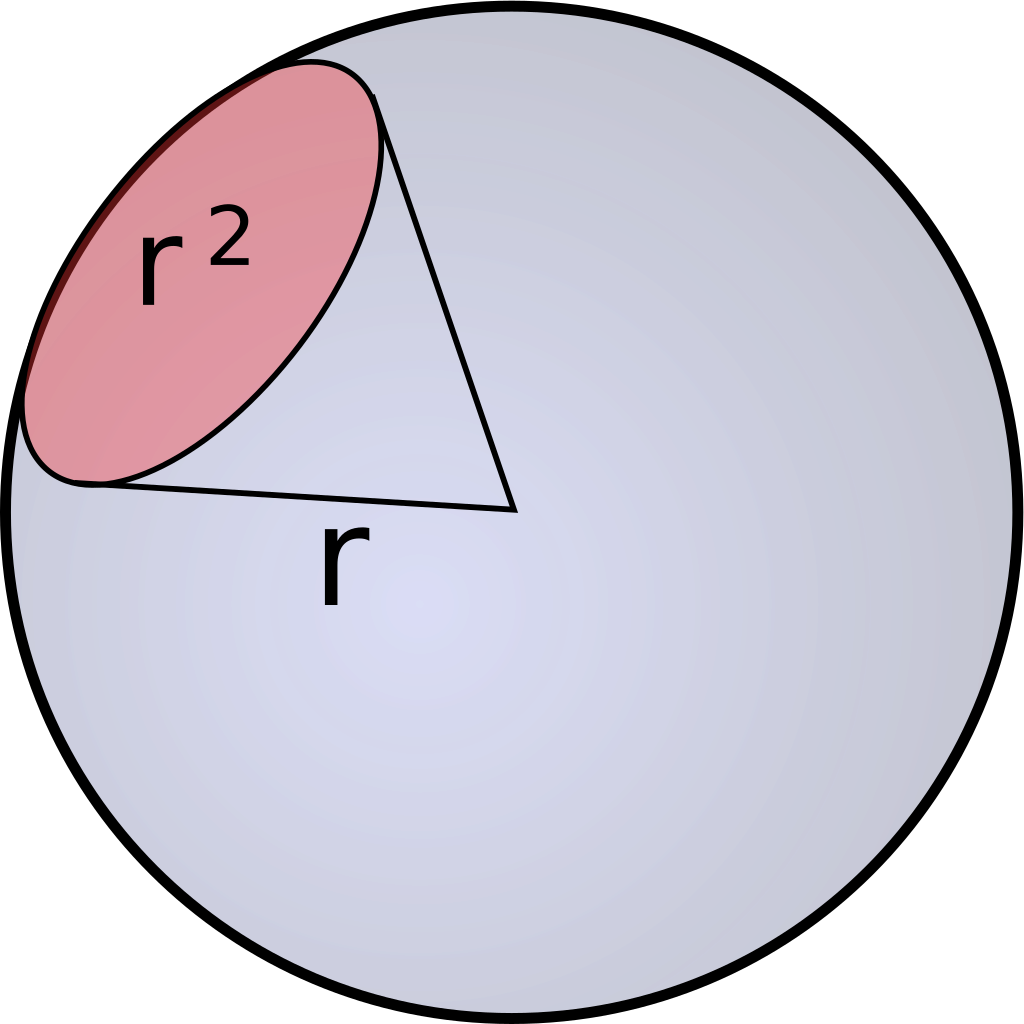
As previously mentioned, Einstein descibres the number of photosinthetically available photons (400-700nm) per square metre per second and is not the SI unit for light intenstiy (luminous flux). The SI unit is lumen, which is described as candela multiplied with the steradian. Candela is the unit for luminous intensity and steradian is the threedimensional equivalent to a twodimensional angle [Figure 1].
Candela and therefore also lumen are not only describing the intensities of different wavelenghts and adding those up, but they are weighing them using the so called lumiosity function [Figure 2].
This function weighs each wavelength depending on how well it is recognized by the human eye and this has huge applications in professional photography.
While this is something that is very useful when working in photography where the recognition of the human eye is important, for photosynthetic purposes this is not useful since photons of various wavelengths can be utilized in a similar way.
The unit Einstein, while not being an SI unit, seems to be the preferable unit for photosynthetic purposes by now, but as previously discussed it is not accurately defined.
Einstein can also be expressed with only SI units as mol of photons of wavelengths between 400 and 700 nm per square meter per second.
In this form, there are no insecurities about the definition and while being more voluminous to write out, we strongly believe it is much preferable.
We are still using einstein as laboratory chargon to communicate more efficiently on a daily basis, however when it comes to scientific publications the SI unit version should be used at all times to circumvent communication errors.
Practical light measurements
In addition to the problems using a non SI unit introduces, the process of of measurement itself is not standardized.
The light intensity could either be measured at the lamp or at the cultures, it can be measured with the cultures inside of the incubator, which yields lower light intensities due to their absorbance, or without the cultures at the place they shall be at once growing.
There are two significantly different devices to measure light intensity, one with a planar sensor and one with a spherical one.
Since the planar sensor has less area and also only measured light from one side it yields lower light intensities than the spherical one.
Depending on the setup and how the planar sensor is used, it can also yield light intensities that are far too high (if pointed at the lamp) or too low (if pointed at e.g. the wall).
The spherical measurement device gives both more reproducable and more accurate light intensities.
There are empirical conversion tables to convert values measured with the planar sensor to values of the spherical measurement and vice versa, but they should be used with great caution.
Again after the valuable input of James Golden we decided to use the spherical sensor to measure the light intensity at any given position.
Light model
Even with the spherical light sensor there are still some difficulties to overcome, for example where to place the cultures for a specific light intensity and that the light intensity has to be measured everytime before a growth curve. To solve both of these problems we decided to build a Light Model that models the light distribution in our incubator. With the help of this model we could enter the exact light intensity we wanted to grow the cultures at and multiple possible places were this light intesity was possible to achieve were given. The source code and the complete documentation how we designed and executed this model can be found on our Modelling page.
Early Growth Curves
HERE THE EARLY GROWTH CURVES AND FACTORIAL PARAMETERS SHALL BE DISCUSSED [TORBEN/BIOLOGIST[ WE ALSO HAVE TO FIT IN A PARAGRAPH ABOUT THE wavelength we measure with With the measurement question for light solved (for us) we started to do growth curves. Many of the publications that we used as templates for our growth curves used specialized cultivation systems that were not at our disposal. With our chosen system (of erlenmeyer flasks in our incubator) there were many adjustable parameters that we stumbled upon once we wanted to do growth curves. Many of these parameters were categorial variables, but there are also some that are numerical values. We decided to do comparative growth curves for these parameters to determine which combination of parameters allows for the best possible doubling time.
Flask Geometry
Fill Volume
Lid Types
Growth Curves Development
HERE THE DEVELOPMENT OF THE CURRENT METHODOLOGY FOR THE GROWTH CURVES IS EXPLAINED [BIOLOGIST]
Growth Curves Model
Variables responsible for growth
As previously described, for categorial differences one can easily do growth curves with all levels of these categories (i.e. the different lids). With this it is possible to determine, at least for the chosen parameters, which level of these categories allows for the fastest growth. In reality, all parameters that play into the growth conditions of the cultures are interlinked and change when other parameters are changed. However, for some parameters the assumption that they do not change upon changing other parameters is probably a fair approximation while drastically reducing the complexity of the investigated problem. Some categorial variables (lid type, number of schikanen in the flask) are probably mostly uncorrelated with other heavily correlated parameters (light intensity, rpm, CO2, temperature) while there are others (total flask volume, filled flask volume, medium) that are more or less correlated with these parameters. While we think that the assumption of no correlation is a fair approximation for the previously mentioned categorial variables, for the fill volume of the flask we do not think it is a good approximation. This variable that as a further approximation we chose to look at as categorical has a big influence on the amount of oxygen and carbon dioxide in the flask. However, since there were already alot of variables we had to take a look at and it is heavily correlated with the CO2 percentage that we are also investigating later, we chose to fix this parameter. This would introduce a (small) error into our model, but it would reduce the complexity and the parameters of oxygen and carbondioxide in our flask can be adjusted with the concentration of carbondioxide in the incubator. For numerical parameters (light intesity, rpm, CO2 %, temperature, filled flask volume) it would also be possible to measure certain values for each variable and use the one that fits best, but there is also the possibility to model the combined effect of these parameters on the doubling time. We did the no correlation assumption of for the previously described categorial variables (lid types, flask geometry, fill volume) and developed based on biological criteria a measurement workflow for other parameters (i.e. how many precultures are used). For four other numerical parameters (temperature, carbondioxide concentration, light intensity and shaker speed) we do think that they are heavily interlinked and decided to investigate them in conjunction with each other. We used the previously established growth curve protocol and collected datapoints varying these four parameters. Due to problems with the incubator and the time constraints going with it we were not able to collect as many datapoints as we would like.
Importance of a mathematical model for growth curve prediction
The data collected is displayed in the following table:
| doubling_time [min] | light_intensity [µmol Photons / m2 * s 400-700 nm] | shaking speed [rpm] | CO2 [%] | temp [℃] | |
|---|---|---|---|---|---|
| 0 | 89.145 | 1500 | 130 | 5 | 41 |
| 1 | 100.014 | 1000 | 220 | 5 | 41 |
| 2 | 99.171 | 1500 | 220 | 5 | 41 |
| 3 | 96.956 | 1800 | 220 | 5 | 41 |
| 4 | 118.375 | 1800 | 130 | 5 | 41 |
| 5 | 113.305 | 1000 | 220 | 5 | 38 |
| 6 | 117.254 | 1500 | 220 | 5 | 38 |
| 7 | 122.141 | 1800 | 220 | 5 | 38 |
| 8 | 77.047 | 1000 | 220 | 3 | 41 |
| 9 | 81.442 | 1500 | 220 | 3 | 41 |
| 10 | 104.293 | 1000 | 220 | 5 | 43 |
| 11 | 96.914 | 1500 | 220 | 5 | 43 |
| 12 | 97.678 | 1800 | 220 | 5 | 43 |
| 13 | 102.040 | 1800 | 220 | 7 | 41 |
| 14 | 110.560 | 1500 | 220 | 7 | 41 |
With this data alone we can highlight the importance to measure these parameters in conjunction with each other. In Figure X there are the doubling times with three different light intensities displayed with either 38°C or 41°C as temperature. While the doubling times for the lower temperature are smaller, also the trend for the light intensity is reverted. For the high temperature the higher the intensity the lower the doubling time while for the low temperature the contrary is the case. This shows that these parameters are not independent of each other and should also be investigated not on their own but in conjunction with each other.


To investigate these parameters in conjunction with each other we decided to build a model that predicts the doubling time based on the investigated parameters.
Boundary behaviour
Something that is not part of our data are the boundaries that naturally exist for growth curves of cyanobacteria. These are partially given be the machines we are using (e.g. the maximal strength of the lamps, the maximum rpm of our shaker) and partially given by the constitution of the cyanobacteria (e.g. the maximal/minimal temperature they can grow at). With our knowledge acquired while handling this cyanobacteria, we decided on the following cutoffs:
| Parameter | Value |
|---|---|
| min light [µmol Photons / m2 * s 400-700 nm] | 100 |
| max light [µmol Photons / m2 * s 400-700 nm] | 3000 |
| min rpm | 30 |
| max rpm | 260/300 |
| min temperature | 30 [℃] |
| max temperature | 50 [℃] |
| min CO2 | 1 |
| max CO2 | 10/20 |
For light and temperature and the lower boundaries of CO2 and rpm we used cutoffs at which we are convinced that no proper growth is possible. For the upper boundaries of CO2 (10) and rpm (260) we used the highgest values that are possible due to the hardware used. For these two boundaries we also tried to increase the values further to not punish the maximal possible values too much but still incentivize our model to not use the values near the booundaries. We added one datapoint for each of these boundaries and used the most common values found in our model for the rest of the values. As example, the datapoint added for the low light and low rpm values are shown in the following table:
| doubling time [min] | light intensity [µmol Photons / m2 * s 400-700 nm] | shaking speed [rpm] | CO2 [%] | temperature [℃] | |
|---|---|---|---|---|---|
| min light | 1000 | 100 | 220 | 5 | 41 |
| min rpm | 1000 | 1500 | 30 | 5 | 41 |
We added a very high doubling time insted of a doubling time of 0 to ensure that our model has the correct behaviour in edge cases. For example, that the model predict an increased doubling time the hotter the temperature gets insted of predicting very low doubling times for those edge cases because we fed it a doubling time of 0. When we entered this data into our model, the performance was drastically reduced. We even experimented with different doubling times that we entered for this sub dataset, but for all cases tried the performance of the model was still worse than without adding this dataset in the first place. Again, due to the small amount of data that we have in the original dataset, if we add these 8 datapoints they have a huge effect on the model even outside of the boundary cases. Due to this decrease in performance we decided to not use this dataset, but we are still convinced that with enough data this would increase the accuracy of the model, especially in boundary cases.
Modelling approach
Due to the small amount of data we were able to collect we decided to use a polynomial regression model instead of a more data demanding approach like k nearest neighbors, support vector machines or neural networks. Even with this approach, the amount of data we have at our disposal is not enough to deliver a model that we would describe as accurate within and especially not outside of our training data. Nevertheless, we think a model like this is the best way forward if we want to properly predict the doubling time and with more data a very accurate model can be built. We used a common approach to polynomial regression models in that we performed a linear regression on nonlinear functions of the data. This means that we use the previously established variables (temp, rpm, light intensity, CO2) and construct the polynomial features of this dataset. For two variables x1 and x2 and a polynomial with the degree 2 this would mean we have the following values as data : [1, x1, x2, x1*x2, x1*x1, x2*x2]. This is possible due to the fact that a linear model is not limited to a linear function but to linear parameters for the variables it builds on. The code used to build this model is shown here :
          import numpy as np
          import pandas as pd
          import sklearn
          import operator
          #from sklearn.cross_validation import train_test_split
          from sklearn.preprocessing import PolynomialFeatures
          from sklearn.linear_model import LinearRegression
          from sklearn.linear_model import LassoCV
          from sklearn.pipeline import Pipeline
          from sklearn.metrics import mean_squared_error, r2_score
          degree_polynomial = 8
          size_test = 1

          data_model = pd.read_csv("data_model_clean_neu.csv")
          data_prep = data_model.drop("Unnamed: 0", axis = 1)


          # Now I want to add data that shows the constraints of the system, so I will engineer fake data to correctly predict everything
          # Format is doubling time, light, rpm, co2, temp
          low_light = [1000,100,220,5,41]
          high_light = [1000, 3000, 220, 5, 41]
          low_rpm = [1000,1500,30,5,41]
          high_rpm = [1000,1500,300,5,41]
          low_co2 = [1000,1500,220,1,41]
          high_co2 = [1000,1500,220,20,41]
          low_temp = [1000,1500,220,5,30]
          high_temp = [1000,1500,220,5,50]

          boundary = []
          boundary.append(high_temp)
          boundary.append(low_temp)
          boundary.append(high_co2)
          boundary.append(low_co2)
          boundary.append(high_rpm)
          boundary.append(low_rpm)
          boundary.append(high_light)
          boundary.append(low_light)
          boundary = pd.DataFrame(boundary)

          boundary.columns = ["doubling_time","light_intensity","rpm","co2","temp"]
          result = pd.concat([boundary, data_prep])

          # Now we need to split the data into x and y
          x = data_prep.drop(["doubling_time"], axis = 1)
          y = data_prep["doubling_time"]


          # To troubleshoot and once we have enough data, this is a very easy and sometimes faulty way to generate a train_test_split
          # For an advanced train test split the sklearn functionality would be used
          x_train = x[:-size_test]
          x_test = x[-size_test:]
          y_train = y[:-size_test]
          y_test = y[-size_test:]

          # Now we define the polynomial and the data that we want to predict
          poly = PolynomialFeatures(degree=degree_polynomial)
          light_pred = [ 1388, 1541, 1750, 1850]
          rpm_pred = [ 147, 147, 147, 147]
          co2_pred = [ 3.8, 3.8, 3.8, 3.8]
          temp_pred = [ 40.5, 40.5, 40.5, 40.5]

          to_predict = pd.DataFrame({"light_pred":light_pred, "rmp_pred":rpm_pred, "co2_pred":co2_pred, "temp_pred":temp_pred})
          to_predict_pol = poly.fit_transform(to_predict)

          #Now the actual model is trained as a pipeline for the polynomial features
          model = Pipeline([('poly', PolynomialFeatures(degree=degree_polynomial)), ('linear', LinearRegression(fit_intercept=True, normalize = True))])
          model = model.fit(x, y)
          #print(model.named_steps["linear"].coef_)
          predictions = model.named_steps["linear"].predict(to_predict_pol)
          #print("hello")
          score = model.score(x_test, y_test)

          # Now the prediction is done and printed together with score and diagnose values for the model
          to_predict = pd.DataFrame(to_predict)
          to_predict["predictions"] = predictions
          print(to_predict)
          print(score)
          print(predictions)

          y_poly_pred = model.predict(x)
          rmse = np.sqrt(mean_squared_error(y,y_poly_pred))
          r2 = r2_score(y,y_poly_pred)
          print(rmse, r2)

          #pred_test = model.predict(x_test)
          #print(pred_test)
          #print(y_test)
          #print(data_prep.to_html())
Again due to the lack of data normal ways of benchmarking the model like train test splits and crossvalidation are not rationally possible. If there would be more data we would use LASSO regression, because this would allow us to eliminate variables that are not useful and avoid a high variance mistake. To showcase how this model using our existing data predicts new data, we decided to predict and measure three new growth curves at unsampled regions within the boundaries of our measurement data. We decided to not calculate the minima that our model predicts, but data that is inside the range of our existing data to properly estimate how well this suboptimal model is working. The predictions of different model versions different only in the degree of polynomials used and the measured doubling time is shown in Figure X.

As we can see in Figure X the prediction quality of the model is poor. The degree of the polynomial is influencing the performance of the model, but there is no clear trend visible. The data for the polynomial degree 3 was excluded since the predictions were negative. The ranking of the different doubling times is the same in all model predictions except for degree 1, with the model predicting the growth curves with the higher light intensities to show a smaller doubling time. However, not only are the predicted doubling time values significantly different from the measured ones, the measured ones are also ranked in a different order (1388>1850>1541>1750). In addition to that the spread of values is higher in the predicted doubling times compared to the measured ones. As expected, the models performance is not good enough to get quantitatively or even qualitatively correct predictions.
Summary and Outlook
WHAT FACTORS DID WE LOOK AT, WHERE IS FURTHER NEED FOR STANDARDIZATION, HOW CAN A STANDARDIZATION BE ACHIEVED [TORBEN/BIOLOGIST]
During this investigation into how to grow UTEX2973 in the optimal way we stumbled upon many things that we thought to be insufficiently documented or standardized.
We investigated how to optimally measure light intensity and thought critically about the state of the art light units.
To make it possible to grow cultures at specific light intensities as well as to make a model of the light intensity in our incubator to help in the everyday life of the wetlab team.
After investigating which wavelength to optimally measure the optical density of our cultures at we started to measure comparative growth curves and developed a reproducable growth curve protocol.
For all parameters that had an effect on the growth curves of UTEX2973 we critically questioned if they could be approximated as independent from other parameters and decided to investigate the temperature, shaking speed, carbon dioxide concentration and light intensity in conjunction with each other.
Since the investigation of four or more different dependent parameters and their effect on the growth is not exhaustively possible for humans we built an easily extendable model that uses polynomial regression to predict the doubling time of various parametercombinations.
However, since measuring a single (or more) doubling time(s) is a very time demanding process, we did not manage to collect a sufficient amount of data to train a model that is able to accurately predict doubling times.
In addition to "just" supplying it with more data, if we have more data more steps can be done to increase the performance of the model.
In addition to a train test split and cross validation to improve the perfomance and decrease the bias of the model towards new data, LASSO regression can be used which would allow to investigate easily how high dimensional the polynome the model is utilizing has to be.
The data we collected was collected only on a couple different levels for each parameter.
While this made it much easier for humans to analyse the data, for the model this drastically reduces its usefulness.
If all datapoints were measured with more randomized values and all datapoints differ on all dimensions of the input data, the data samples the given range much more equally.
With data like that a model can be built that is more robust due to the better sampling of the input space.
A visual representation of the sampling in the rpm
However, for many of the parameters we cannot do that in one measurement, since the rpm, CO2 concentration and temperature has to be identical.
For the light intensity there could have been more sampling which would have improved the performance of the model.
https://static.igem.org/mediawiki/2019/3/39/T--Marburg--model_gridbased_screening.png
References
Ungerer, J., Wendt, K. E., Hendry, J. I., Maranas, C. D., & Pakrasi, H. B. (2018). Comparative genomics reveals the molecular determinants of rapid growth of the cyanobacterium Synechococcus elongatus UTEX 2973. Proceedings of the National Academy of Sciences, 115(50), E11761-E11770.Russo, D. A., Zedler, J. A. Z., Wittmann, D. N., Möllers, B., Singh, R. K., Batth, T. S., ... & Jensen, P. E. (2019). Expression and secretion of a lytic polysaccharide monooxygenase by a fast-growing cyanobacterium. Biotechnology for biofuels, 12(1), 74.