Math modelling

Overview

The following modelling has been considering an in-vitro system. We divide the modelling part into 3 separate sections.

Phagocytosis: We model the dynamics of the process of phagocytosis through which our genetically modified organism (GMO) enters the macrophage. We aim to find the number of GMOs in the Macrophage at a steady state. This result will be used in the iron chelation modelling.
Nitric oxide sensor: We simulate our genetic circuit to test its sensitivity towards different concentrations of Nitric Oxide and to see the response time of our circuit to the environment of the Macrophage.
Iron chelation: We simulate how a Leishmania-infected Macrophage will behave when we introduce our GMO into the system. we vary the production rate of Aerobactin and observe the decrease in iron in the Macrophage.

Phagocytosis

Nitric oxide sensor

Iron chelation

Click on the buttons above to view the individual modules

Phagocytosis

Modelling of Phagocytosis of the GMO by the Macrophage:

Our system has been modelled in vitro. The GMO will be inserted in a Macrophage culture and will enter the macrophage by the process of phagocytosis. We model the dynamics of the GMO entering the Macrophage using a 3 compartment system $A$,$B$ and $C$.
$A$ : The GMOs adherent to the cell membrane of the Macrophage
$B$ : The GMOs that has been phagocytosed
$C$ : The phagocytosed GMOs that fuse with the lysosome (death of the GMO)

$$ \stackrel{R_a}\rightarrow A \stackrel{k_i}\rightarrow B \stackrel{k_f}\rightarrow C $$

The GMO present outside the Macrophage first adheres to the surface of the Macrophage and then the Macrophage engulfs these adherent bacteria (phagocytosis). The GMOs are now inside phagosomes. These phagosomes eventually fuse with the lysosome causing the death of our GMO. Our GMO will be active while it is in compartment B therefore we focus on the population of our GMO in this compartment.

Let $B_a$ , $B_b$ and $B_c$ be the population of our GMO in the compartments A ,B and C respectively. We assume first order kinetics, therefore we can write the following differential equations:

$$\frac{dB_a}{dt} \space = \space -K_i B_a \space + \space R_a $$ $$\frac{dB_b}{dt} \space = \space K_i B_a \space - \space K_f B_b$$ $$\frac{dB_c}{dt} \space = \space K_f B_b$$

Where, $ \space R_a$ is the rate of adherence of our GMO to the surface of the Macrophage $K_i$ is the rate of intake of GMO into the macrophage $K_f$ is the rate of uptake of the GMO by lysosomes (death of the GMO)

For Peritonial Macrophages we have the values:$^{[1]}$
$ R_a \space = \space 0.011 \space \space No. \space of \space GMO \space per \space cell/min $ ( $t<$ $15 min$)
$ 0.002 \space \space No. \space of \space GMO \space per \space cell/min $ ( $t>$ $15 min$ )
$K_i \space = \space 0.047 \space \space min^{-1} $
$K_f \space = \space 0.109 \space \space min^{-1} $

Using these values we get the following graph from our simulation:

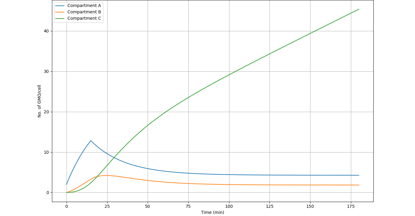
Figure 1 - Time evolution of the populaton of our GMO in the various compartments.

Results

The system achieves steady state in 120 to 150 minutes in compartment A ($4.26 \space $ GMOs$ \space per \space macrophage$) and compartment B ($1.82 \space $ GMOs$ \space per \space macrophage$)
In the steady state, there are approximately 2 active GMOs per macrophage. This data will be utilised in the Iron regulation modelling.

References

Bizal, C. L., Butler, J. P., Feldman, H. A. and Valberg, P. A. (1991), Kinetics of Phagocytosis and Phagosome‐Lysosome Fusion in Hamster Lung and Peritoneal Macrophages. J Leukoc Biol, 50: 229-239. doi:10.1002/jlb.50.3.229

Nitric oxide sensor

The most integral part of the project is the Nitric Oxide ($NO$) sensor. The genetic circuit is designed to operate in a narrow band of $NO$ concentration. Ideally, the circuit should be active between 2 concentrations $C_1$ and $C_2$. $C_1$ is the concentration slightly greater than the normal Nitric Oxide concentration of an uninfected Macrophage (which is around $1 \space \mu M \space ^{[1]}$). $C_2$ is the concentration slightly less than the concentration of Nitric Oxide inside an infected Macrophage (which is around $7-28 \space \mu M \space ^{[1]}$). It is important to test the circuit using a model in order to check for viability and to give useful insights to the wet lab team.

Figure 1 - The Nitric Oxide Sensing Module

Main Goals of this Model

To see the activity of the genectic circuit under various Nitric Oxide concentrations/ To test the sensitivity of the Nitric Oxide Sensor
To identify the parameters that can be tuned to get the desired Nitric Oxide sensing range
To test the response time of our circuit to the environment of the Leishmania infected Macrophage
To suggest improvements that can be made to our circuit to create a better sensor.

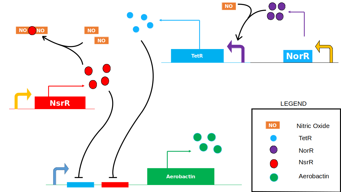
To model the Genetic Circuit, we first consider the various reactions and interactions involved:

$NorR$ and $NsrR$ are protiens that sense Nitric oxide. Nitric oxide binds with $NorR$ and $NsrR$ to form their respective complexes. The $NorR-NO$ complex further acts as an activator for the production of $TetR$. $NsrR$ and $TetR$ bind to the $NsrR-binding-site \space $ and $TetR-binding-site \space $ respectively at the operator region of our Aerobactin producing part. Hence, $NsrR$ and $TetR$ repress the production of Aerobactin.

$$ NsrR + NO \underset{k_{b_1}}{\stackrel{k_{f_1}}{\rightleftharpoons}} NsrR-(NO) $$ $$ NsrR-(NO) + NO \underset{k_{b_2}}{\stackrel{k_{f_2}}{\rightleftharpoons}} NsrR-(NO)_2 $$ $$ NorR + NO \underset{k_{b_3}}{\stackrel{k_{f_3}}{\rightleftharpoons}} NorR-NO $$

The kinetic equations for the above reactions can be written as follows: $$r_1 \space = \space k_{f_1}[NsrR][NO] - k_{b_1}[NsrR-(NO)] $$ $$r_2 \space = \space k_{f_2}[NsrR-(NO)][NO] - k_{b_2}[NsrR-(NO)_2] $$ $$r_3 \space = \space k_{f_3}[NorR][NO] - k_{b_3}[NorR-(NO)]$$

We can express the rate of change of concentrations as follows: $$\frac{d[NsrR]}{dt} \space = \space \beta_{NsrR} \space - \space \alpha_{NsrR} [NsrR] - \space r_1$$ $$\frac{d[NorR]}{dt} \space = \space \beta_{NorR} \space - \space \alpha_{NorR} [NorR] - \space r_3$$ $$ \frac{d[TetR]}{dt} \space = \space \frac{\beta_{TetR}}{1 \space + \space \frac{K_{Tet}}{[NorR-(NO)]^2}} \space - \space \alpha_{TetR} [TetR]$$ $$\frac{d[NsrR-(NO)]}{dt} \space = \space r_1 - \space \alpha_{NsrR-(NO)} [NsrR-(NO)]$$ $$\frac{d[NsrR-(NO)_2]}{dt} \space = \space r_2 \space - \space \alpha_{NsrR-(NO)_2} [NsrR-(NO)_2]$$ $$\frac{d[NorR-(NO)]}{dt} \space = \space r_3 \space - \space \alpha_{NorR-(NO)} [NorR-(NO)]$$

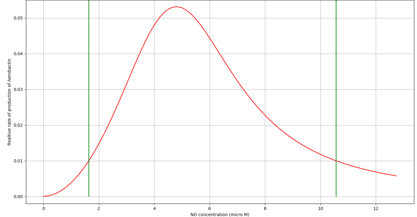
The rate of production ($r_{Ab}$) of our Iron Chelator, Aerobactin( $Ab$), at any time instant can be expressed as: $$ \space r_{Ab} \space = \space \frac{\beta_{Ab}}{1 \space + \space \frac{[NsrR]^2}{K_{D_1}} \space + \space \frac{[TetR]^2}{K_{D_2}}}$$ Or the Relative rate of production ($f_{Ab}$) can be given by: $$ \space f_{Ab} \space = \space \frac{r_{Ab}}{\beta_{Ab}} \space = \space \frac{1}{1 \space + \space \frac{[NsrR]^2}{K_{D_1}} \space + \space \frac{[TetR]^2}{K_{D_2}}}$$

The relative rate of production of Aerobactin ($f_{Ab}$ tells us how the  and  system affects the rate of production of Aerobactin. Therefore we focus on $f_{Ab}$ in this model of our Nitric Oxide Sensor. We will focus more on rate of production of Aerobactin in the Iron Chelation Model.

Parameters

The table of parameters used for the simulation ( * = assumed)
Parameter	Description	Value	Unit	Source
$k_{f_1}$	$NsrR-(NO)$ production rate	$271.2$	$\mu M ^{-1} \space min^{-1}$	[2]
$k_{b_1}$	$NsrR-(NO)$ dissociation rate	$100$	$min^{-1}$	[2]
$k_{f_2}$	$NsrR-(NO)_2$ production rate	$6.78$	$\mu M ^{-1} \space min^{-1}$	[2]
$k_{b_2}$	$NsrR-(NO)_2$ dissociation rate	$100$	$min^{-1}$	[2]
$k_{f_3}$	$NorR-(NO)$ production rate	$1.1183$	$\mu^{-1}min^{-1}$	[3]
$k_{b_3}$	$NorR-(NO)$ dissociation rate	$0.0363665$	$min^{-1}$	[3]
$\alpha_{NsrR}$	Degradation rate of $NsrR$	$0.0015$	$min^{-1}$	[4]
$\alpha_{NorR}$	Degradation rate of $NorR$	$89.159$	$min^{-1}$	[2]
$\alpha_{TetR}$	Degradation rate of $TetR$	$0.0348$	$min^{-1}$	*
$K_{Tet}$	Activation rate of $TetR$	$0.5×10^{-4} $	$\mu M^2$	*
$\alpha_{NsrR-(NO)}$	Degradation rate of $NsrR-(NO)$	$1$	$min^{-1}$	*
$\alpha_{NsrR-(NO)_2}$	Degradation rate of $NsrR-(NO)_2$	$1$	$min^{-1}$	*
$\alpha_{NorR-(NO)}$	Degradation rate of $NorR-(NO)$	$0.0363665$	$min^{-1}$	[2]

Tunable Parameters

The expression rates of $NorR$, $NsrR$ and $TetR$
The binding affinities of $NsrR$ and $ TetR$ to their respective binding sites.

How can such tuning be achieved?

Expression rates of genes: There are 2 possible ways of tuning the expression rates of any particular gene.
- By inducing mutations in the promoter region of the gene that will alter its affinity towards RNA Polymerase in turn altering the rate of transcription and translation.
- By using the promoter regions of other known genes having transcription rates in the desired range.
To get any desired expression rate, a combination of the above 2 methods could be used.
Binding of $TetR$ and $NsrR $ to their respective binding sites (Operator region): This can be achieved using the followiing ways:
- Inducing mutations in the operator region so as to alter the affinities of the repressors to the binding sites.
- Inducing mutations in the repressor protiens by mutating the coding region that are responsible for producing these protiens. Hence, changing their affinities to the operator site.

Tuning the circuit

Objective: To tune the circuit so that its activity is maximum between $NO$ concentration of $C_1$ and $C_2$.
What parameters control the activity of the genetic circuit at different concentrations of $NO$?

Since $TetR$ starts repressing the production of our Iron chelator, Aerobactin( $Ab$), after a certain concentration of $NO$, it is evident that the parameters associated with the $TetR$ system, control the higher bound of the circuit's active region (the concentration range of $NO$ for which the expression of Aerobactin is maximum).
Similarly, the $NsrR$ represses the expression of Aerobatin at lower concentrations of $NO$. Therefore, the parameters associated with the $NsrR$ system will control the lower bound of the active region of our circuit.

We tuned the parameters of the $TetR$ and the $NsrR$ system so that the circuit is active between $C_1$ and $C_2$ concentrations of $NO$. We got the following results:

Figure 2 - Relative rate of production of Aerobactin (steady state) vs Nitric oxide $[NO]$. The active region of our circuit lies between $\approx1.5\mu M$ to $\approx10.5\mu M$

The tuned parameters for the genetic circuit (Figure 1)
Parameter	Description	Value	Unit
$\beta_{NsrR}$	Constitutive rate of production of $NsrR$	$7$	$\mu M \space min^{-1}$
$\beta_{NorR}$	Constitutive rate of production of $NorR$	$1$	$\mu M \space min^{-1}$
$\beta_{TetR}$	Maximum rate of production of $TetR$	$7.93$	$\mu M \space min^{-1}$
$K_{D_1}$	Equilibrium constant of $NsrR$ repression	$0.01225$	$\mu M^2$
$K_{D_2}$	Equilibrium constant of $TetR$ repression	$0.3136$	$\mu M^2$

How long does it take for our circuit to respond to the environment inside a Leishmania infected Macrophage?

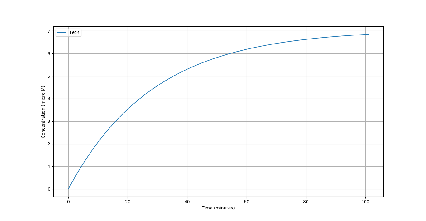
We simulated our circuit for around 100 minutes. Taking $[NO]= 5 \mu M$ as it lies in the middle of active region of our Nitric Oxide sensor. The time evolution of the different components of our system can be seen below:

Figure 2 (a-left),(b-right) - Time evolution of the $NsrR$ system with $[NO]=5 \mu M$. (a) shows the initial behaviour of the system (0-3 min) and (b) shows the steady state behaviour (0-100min) .

Figure 4 - Time evolution of the $NorR$ system with $[NO]=5 \mu M$

Figure 5 - Time evolution of the $TetR$ with $[NO]=5 \mu M$

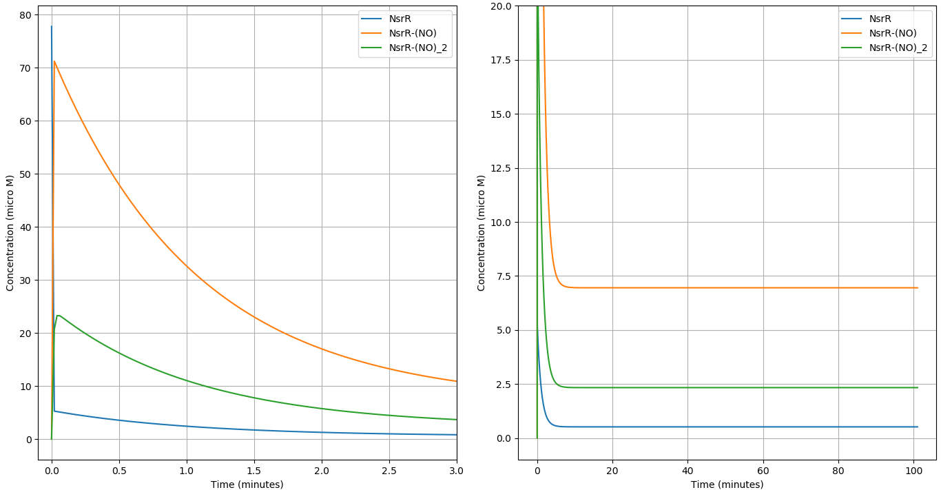
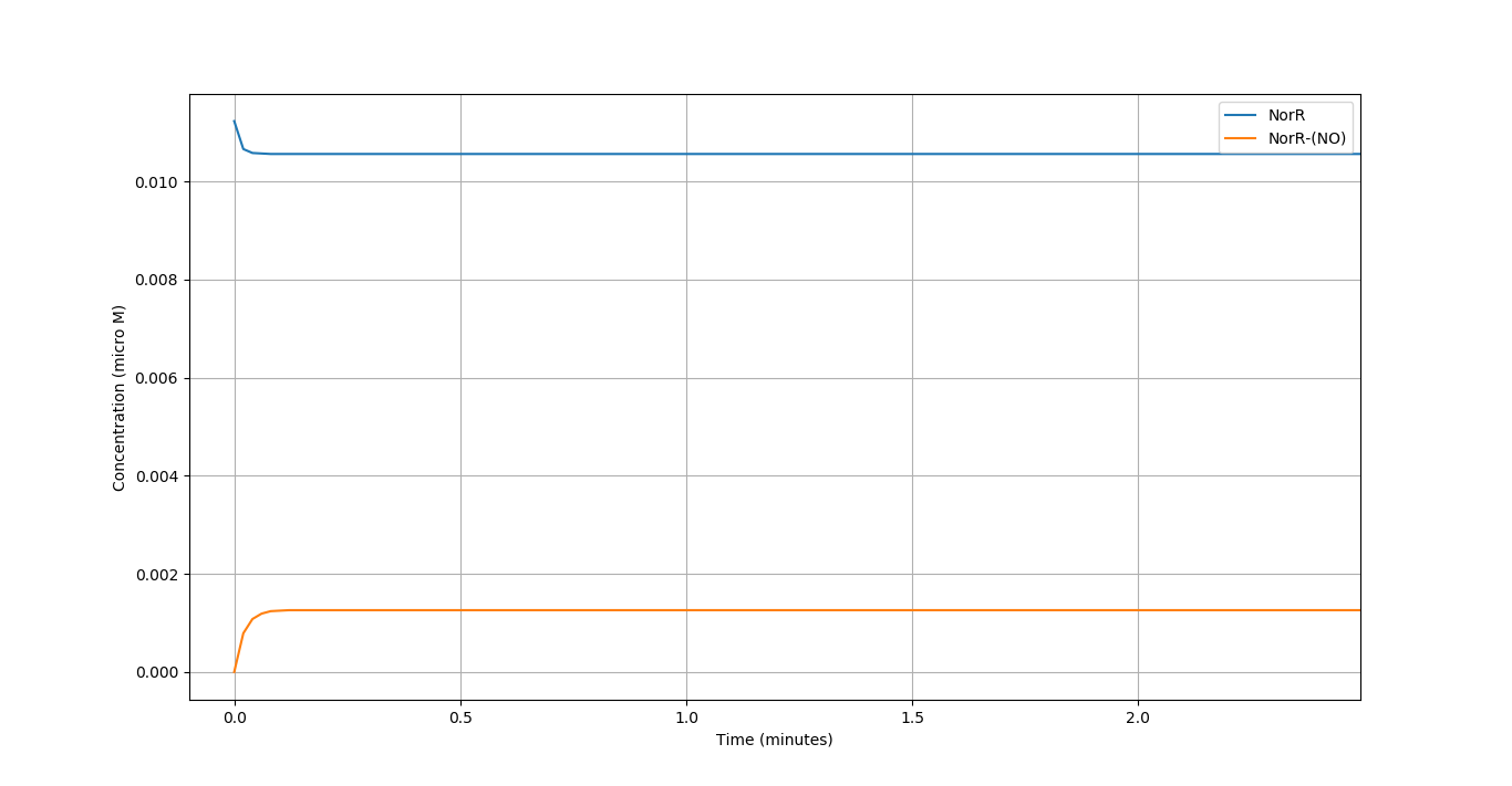
We compare the respone of the circuit for 3 different concentrations of $NO$ in terms of the $f_{Ab}$ vs Time.

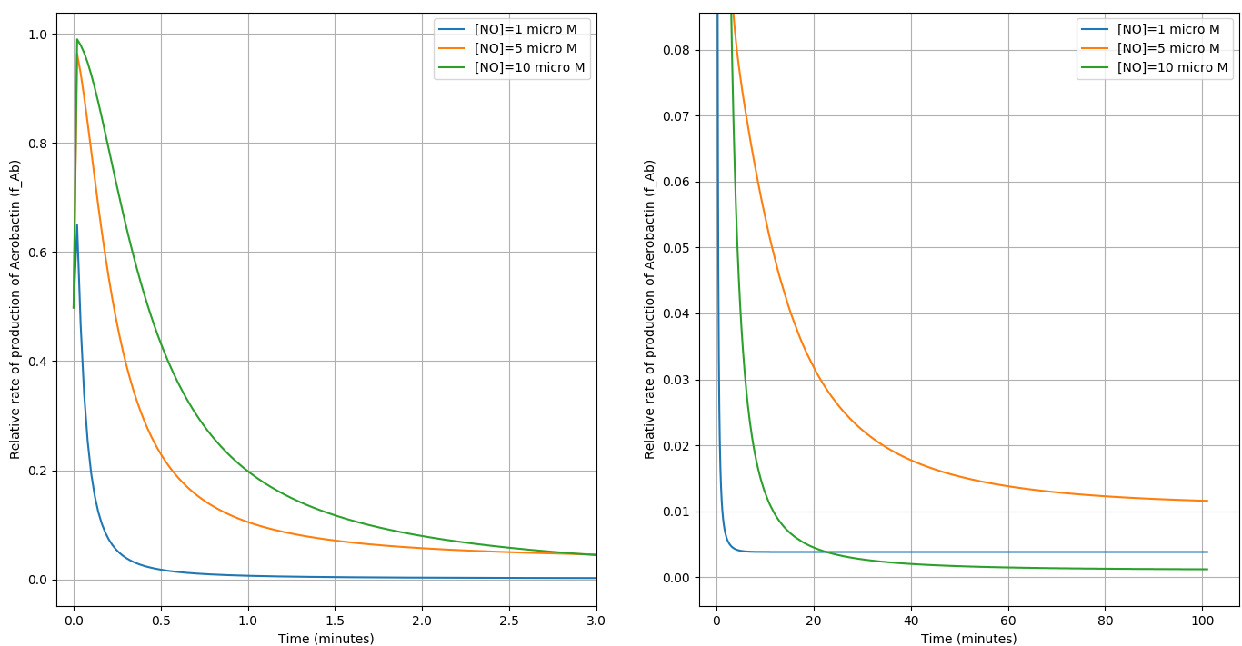
Figure 6 (a-left),(b-right) - The Relative rate of production of $Ab$ vs Time for 3 different concentrations of $NO$.
(a) shows the initial behaviour of the system (0-3 min) and (b) shows the steady state behaviour (0-100min)

Results:

We obtained 2 important results from this model:

The circuit is activated within the $NO$ concentration range of $C_1$ and $C_2$.
The circuit responds to the Macrophage environment almost instantaneously and reaches steady state in $\approx 100$ minutes.
We successfully demonstrated the feasibility of $NsrR$ as $NO$ detector 1 and $NorR$ as $NO$ detector 2 as described in the Design part of our project.

Possible improvements to the Nitric Oxide Sensor

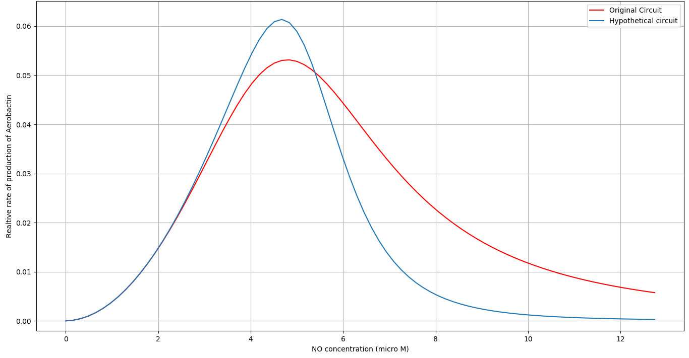
To create a better sensor, the sensitivity of the circuit should be very specific around the concentrations $C_1$ and $C_2$ of $NO$. Ideally, the rate of Aerobactin production should change very steeply at the boundary regions of the active region of the circuit ($NO$ concentration). The factor that controls the sensitivity of the circuit is the number of molecules of the substrate binding to the other reactant in any reaction (cooperativity). This factor is equivalent to the Hill coefficient. It's well known that higher hill coefficient gives better sensitivity (steep change in the graphs).

We simulated a slightly modified circuit with a hypothetical protein having cooperativity factor of $2$ with $NO$ as a replacement of $NorR$ in our genetic circuit. We observed that the circuit was much more sensitive to $NO$ concentration at the upper bound of the active region of our circuit. See figure below:

Figure 7 - Comparing the activity of the Original Nitric Oxide Sensor with the hypothetical one.

We gave these insights to the wet lab team. They started looking for possible replacements for $NorR$ by looking for proteins having higher cooperativity with $NO$. They found another $NO$ sensing protein ($SoxR$) which has cooperativity of 4 with Nitric Oxide. The Wet lab team then developed a part which they attempted to characterize but failed to do so due to unsuccessful attempts at transformation.

References

Aldridge, Christopher & Razzak, Anthony & Babcock, Tricia & Helton, william & Espat, N.. (2008). Lipopolysaccharide-Stimulated RAW 264.7 Macrophage Inducible Nitric Oxide Synthase and Nitric Oxide Production Is Decreased by an Omega-3 Fatty Acid Lipid Emulsion. The Journal of surgical research. 149. 296-302. 10.1016/j.jss.2007.12.758.
Crack, J. C., Svistunenko, D. A., Munnoch, J., Thomson, A. J., Hutchings, M. I., & Brun, N. E. L. (2016). Differentiated, Promoter-specific Response of [4Fe-4S] NsrR DNA Binding to Reaction with Nitric Oxide. Journal of Biological Chemistry, 291(16), 8663–8672. doi: 10.1074/jbc.m115.693192
iGEM ETH Zurich, 2016
iGEM Edinburgh, 2009

Iron chelation

In this model, we plan to investigate the hypothesis of eliminating Leishmania parasites by restricting its growth by chelating iron inside the Macrophage. From literature surveys and interviews with experts, we got a positive response for this method of elimination and we plan to verify this fact by our modelling.

Iron intake in macrophages and many other cells are tightly controlled by a core regulatory network that contains several intertwined feedback loops and includes the key regulatory mechanisms of iron homeostasis.

The key task of intracellular iron homeostasis is to tightly control the level of the so-called labile Iron pool ($LIP$), the collection of weakly bound Iron in the cell $^{[1]}$, which is available for a variety of interactions with other molecules. The parasite can tune this regulation to its liking to intake Iron from the $LIP$.

We use a simplistic model to describe the Iron Chelation ignoring components like Ferritin, which sequesters excess Iron in the system, as we will be working with an Iron deficient system.

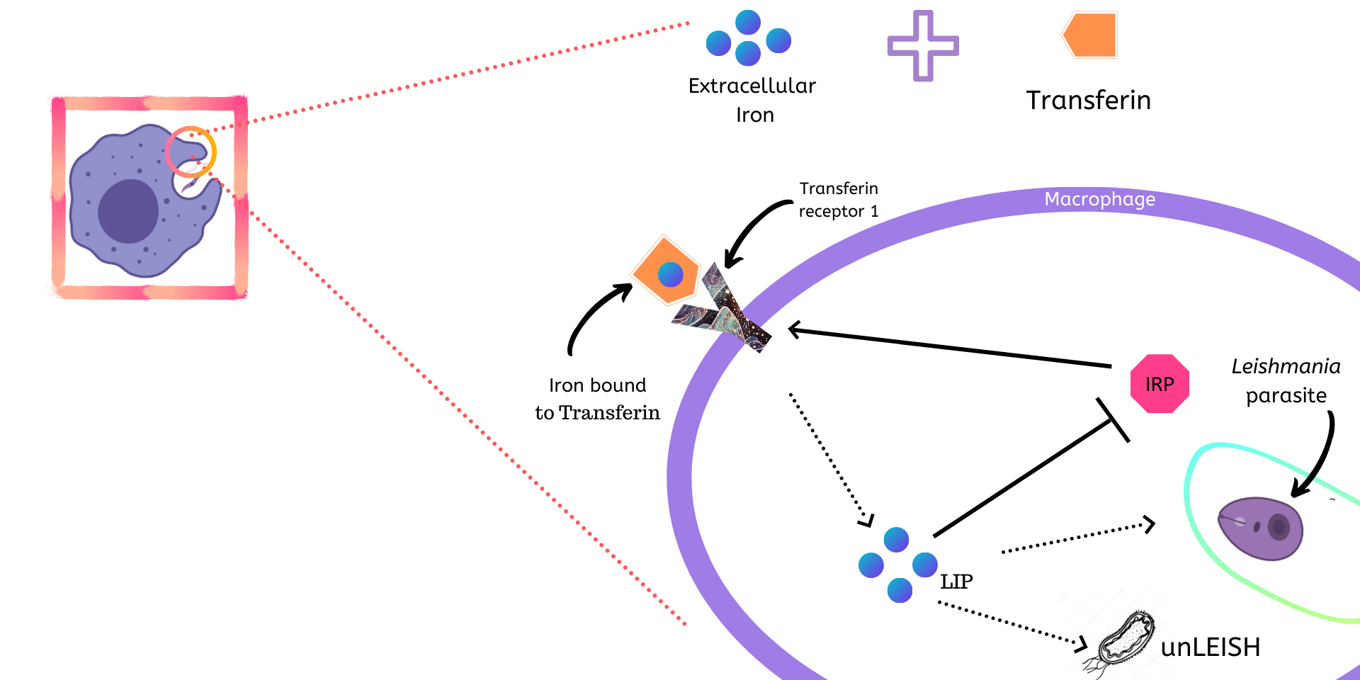
Components of the System

Transferrin-bound-Iron ($TfFe$) is the extracellular Iron bound to Transferrin, which is an Iron transporting protein.
Transferrin Receptor 1 ($TfR1$) is required for Iron import from Transferrin into cells by endocytosis and is present on the exterior surface of the macrophage.
Iron Regulatory Proteins ($IRP$) is an IRE(Iron Responsive Element)-binding protein involved in the control of Iron metabolism. In this model, it activates production of $TfR1$.
Labile Iron Pool ($LIP$): An intracellular pool of nonprotein bound accessible Iron ions inside the macrophage. This represses production of $IRP$s.
Leishmania parasites
Aerobactin ($Ab$): Iron chelator

Assumptions

We assume that the system has reached steady state with the parasite present inside and there is no export of iron outside the system, because it has been observed that Leishmania donovani inhibits ferroportin translation, the protein responsible for export of iron inside the host macrophage$^{[3]}$.
In our model, any concentration of iron that is imported is completely in the labile iron pool ($LIP$).
Leishmania intakes iron from the $LIP$ at a constant rate.

Therefore, this section is broken into 3 parts:

Finding Steady state condition for the system ( Leishmania-infected macrophage )
Studying the influence of chelation of Iron by our GMO in this system.
Determination of an effective production rate of Aerobactin

1) Finding Steady state condition for the system (Leishmania-infected macrophage)

Figure 1 - The *Leishmania*-infected macrophage system

The ODEs that describes the system: $$ \frac{d[TfR1]}{dt} \space = \space \alpha_{TfR1} \frac{[IRP]}{k_{TfR1} \space + \space [IRP]} \space - \space \gamma_{TfR1} [TfR1]$$ $$ \frac{d[IRP]}{dt} \space = \space \alpha_{IRP} \frac{k_{IRP}}{k_{IRP} \space + \space [LIP]} \space - \space \gamma_{IRP} [IRP] $$ $$ \frac{d[LIP]}{dt} \space = \space k_{LIP} [TfFe][TfR1] \space - \space \gamma_{LIP}[LIP] \space - \space k_{Leish} C_L $$

Table 1 ( * = assumed )
Parameters	Description	Value	Unit	Reference
$\alpha_{TfR1}$	Maximum production rate of $TfR1$	$2\times 10^{-11}$	$Msec^{-1}$	[2]
$\alpha_{IRP}$	Maximum production rate of $IRP$	$2\times 10^{-11}$	$Msec^{-1}$	[2]
$k_{LIP}$	Iron import rate of $TfR1$	$2\times 10^{3}$	$M^{-1}sec^{-1}$	*
$k_{TfR1}$	Activation coefficient of $TfR1$	$1\times 10^{-6}$	$M$	[2]
$k_{IRP}$	Activation coefficient of $IRP$	$1\times 10^{-6}$	$M$	[2]
$\gamma_{TfR1}$	Degradation rate of $TfR1$	$8.37\times 10^{-6}$	$sec^{-1}$	[2]
$\gamma_{IRP}$	leakage rate of $IRP$	$1.59\times 10^{-5}$	$sec^{-1}$	[2]
$k_{Leish}$	Rate of iron intake from the $LIP$ by Leishmania	$1$	$sec^{-1}$	*
$C_L$	Concentration of Leishmania inside the macrophage	$1.328\times 10^{-9}$	$M$	4 parasites per macrophage

For the simulation, we take $[TfFe] \space = \space 2 \mu M$
We find the steady state concentrations for $LIP$, $TfR1$, $IRP$. (Table below)

Table 2
Component	Steady state concentration	Unit
$LIP$	$2.713\times10^{-6}$	$M$
$TfR1$	$6.034\times10^{-7}$
$IRP$	$3.381\times10^{-7}$

2) Studying the influence of Iron chelation by our GMO

Figure 2 - The *Leishmania*-infected macrophage system with GMO present inside

Now, we introduce our GMO into the macrophage at $t=1000$ minutes. From our phagocytosis modelling, we found that $\approx 2$ GMOs will survive inside the macrophage. We model the chelation using the following reaction: $$ LIP \space + \space Ab \stackrel{k}\rightarrow \space (LIP-Ab)_{Complex} $$

The ODEs describing the system now are: $$ \frac{d[TfR1]}{dt} \space = \space \alpha_{TfR1}\frac{[IRP]}{k_{TfR1} + [IRP]} \space - \space \gamma_{TfR1}[TfR1] $$ $$ \frac{d[IRP]}{dt} \space = \space \alpha_{IRP}\frac{k_{IRP}}{k_{IRP}+[LIP]} \space - \space \gamma_{IRP}[IRP] $$ $$ \frac{d[LIP]}{dt} \space = \space k_{LIP}[TfFe][TfR1] \space - \space \gamma_{LIP}[LIP] \space - \space k_{Leish}C_L \space - \space k[Ab][LIP] $$ $$ \frac{d[Ab]}{dt} \space = \space n \cdot r_{Ab} \space - \space \alpha_{Ab}[Ab] \space - \space k[Ab][LIP] $$ Where, $n$ is the number of GMOs inside the Macrophage $r_{Ab}$ is the rate of production of $Ab$, $\alpha_{Ab}$ is the rate of degradation of $Ab$ and $k$ is the chelation rate of Iron by $Ab$. We take $n=2$ (from Phagocytosis modelling).

With these parameter values and conditions (Table 1 and 2), we evolve the system with an $r_{Ab}=5×10^{-8} M \space sec^{-1}$

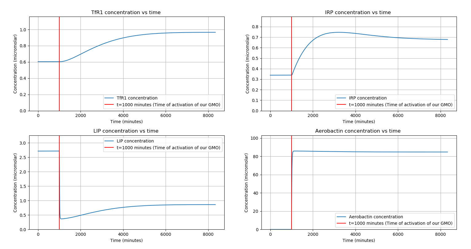
Time evolution of each component of the system

We observe that there is a significant decrease in $LIP$ concentration ($\approx 68 \% $), while all other proteins reacted to the presence of Aerobactin inside the macrophage in accordance with our hypothesis.

3) Determination of an effective production rate of Aerobactin

The main goal of Iron chelation is to make Leishmania starve of its essential Iron requirements and eventually killing it. Therefore, we must tune our circuit so that it chelates just enough Iron so as to inhibit Leishmania growth and eventually eliminate it. Therefore, by knowing the minimum decrease in concentration of $LIP$ that would kill Leishmania, we can estimate the rate of production of Aerobactin required to achieve it.

We would like to study how a change in the production rate of Aerobactin affects the percentage decrease in $LIP$ concentration. This will help us in tuning the rate of production of Aerobactin to achieve the desired decrease in $LIP$ concentration. We obtained the following results for steady-state $LIP$ concentration for various rates of production of Aerobactin:

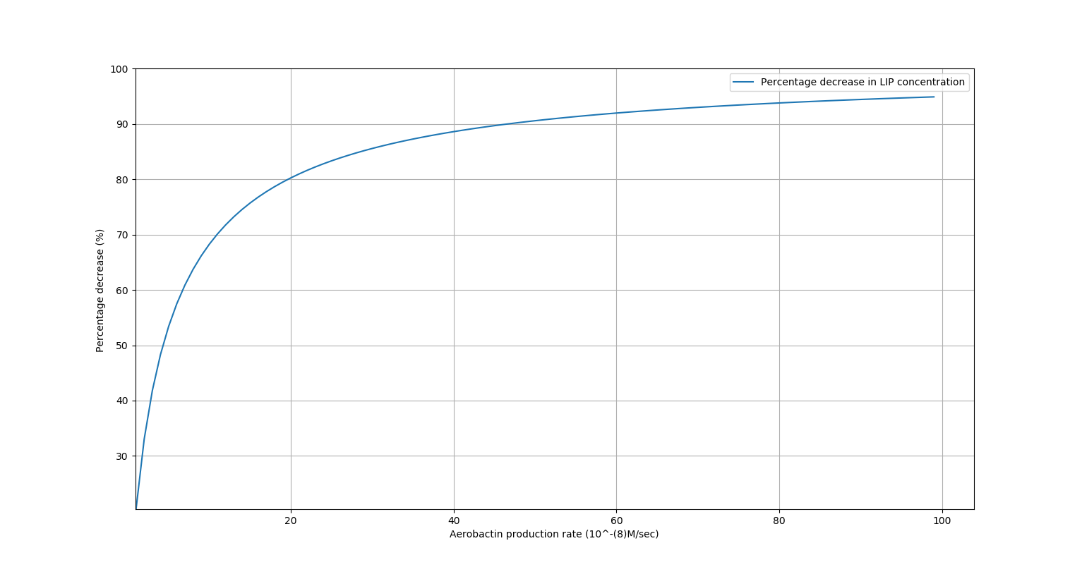
Figure 3 - Decrease in LIP concentration vs Rate of production of Aerobactin ($r_{Ab}$)

Table 3
Percentage decrease in $[LIP] \space \space $(%)	$r_{Ab}$ ($\mu M/min$)
$50$	$1.8$
$60$	$2.4$
$70$	$3.6$
$80$	$6.0$
$90$	$14.4$

Results

We observe that on increasing production rate of Aerobactin, the percentage decrease in $[LIP]$ saturates to near about 100%. This confirms the hypothesis that using a chelator, even with a regulation system, can decrease Iron concentration significantly. Also, our wet lab experiments have confirmed that decreasing iron concentration in the vicinity of the Leishmania parasite inhibits its growth.

Therefore, if we were to find the minimum percentage decrease in LIP concentration that results in Leishmania elimination, this model can evaluate the production rate of Aerobactin ($r_{Ab}$) that our GMO needs to produce.

In conclusion, we have shown that using a chelator, we can restrict the growth of Leishmania parasites. Also, we can predict a suitable $r_{Ab}$ for our GMO to do so.

References

Chifman, J., Kniss, A., Neupane, P., Williams, I., Leung, B., Deng, Z., … Laubenbacher, R. (2012). The core control system of intracellular iron homeostasis: a mathematical model. Journal of theoretical biology, 300, 91–99. doi:10.1016/j.jtbi.2012.01.024
Mitchell S, Mendes P (2013) A Computational Model of Liver Iron Metabolism. PLoS Comput Biol 9(11): e1003299. https://doi.org/10.1371/journal.pcbi.1003299
Ben-Othman R, Flannery AR, Miguel DC, Ward DM, Kaplan J, et al. (2014) Leishmania-Mediated Inhibition of Iron Export Promotes Parasite Replication in Macrophages. PLOS Pathogens 10(1): e1003901. https://doi.org/10.1371/journal.ppat.1003901

Parameter	Description	Value	Unit	Source
\(k_{f_1}\)	\(NsrR-(NO)\) production rate	\(271.2\)	\(\mu M ^{-1} \space min^{-1}\)	[2]
\(k_{b_1}\)	\(NsrR-(NO)\) dissociation rate	\(100\)	\(min^{-1}\)	[2]
\(k_{f_2}\)	\(NsrR-(NO)_2\) production rate	\(6.78\)	\(\mu M ^{-1} \space min^{-1}\)	[2]
\(k_{b_2}\)	\(NsrR-(NO)_2\) dissociation rate	\(100\)	\(min^{-1}\)	[2]
\(k_{f_3}\)	\(NorR-(NO)\) production rate	\(1.1183\)	\(\mu^{-1}min^{-1}\)	[3]
\(k_{b_3}\)	\(NorR-(NO)\) dissociation rate	\(0.0363665\)	\(min^{-1}\)	[3]
\(\alpha_{NsrR}\)	Degradation rate of \(NsrR\)	\(0.0015\)	\(min^{-1}\)	[4]
\(\alpha_{NorR}\)	Degradation rate of \(NorR\)	\(89.159\)	\(min^{-1}\)	[2]
\(\alpha_{TetR}\)	Degradation rate of \(TetR\)	\(0.0348\)	\(min^{-1}\)	*
\(K_{Tet}\)	Activation rate of \(TetR\)	\(0.5×10^{-4} \)	\(\mu M^2\)	*
\(\alpha_{NsrR-(NO)}\)	Degradation rate of \(NsrR-(NO)\)	\(1\)	\(min^{-1}\)	*
\(\alpha_{NsrR-(NO)_2}\)	Degradation rate of \(NsrR-(NO)_2\)	\(1\)	\(min^{-1}\)	*
\(\alpha_{NorR-(NO)}\)	Degradation rate of \(NorR-(NO)\)	\(0.0363665\)	\(min^{-1}\)	[2]

Parameter	Description	Value	Unit
\(\beta_{NsrR}\)	Constitutive rate of production of \(NsrR\)	\(7\)	\(\mu M \space min^{-1}\)
\(\beta_{NorR}\)	Constitutive rate of production of \(NorR\)	\(1\)	\(\mu M \space min^{-1}\)
\(\beta_{TetR}\)	Maximum rate of production of \(TetR\)	\(7.93\)	\(\mu M \space min^{-1}\)
\(K_{D_1}\)	Equilibrium constant of \(NsrR\) repression	\(0.01225\)	\(\mu M^2\)
\(K_{D_2}\)	Equilibrium constant of \(TetR\) repression	\(0.3136\)	\(\mu M^2\)

Parameters	Description	Value	Unit	Reference
\(\alpha_{TfR1}\)	Maximum production rate of \(TfR1\)	\(2\times 10^{-11}\)	\(Msec^{-1}\)	[2]
\(\alpha_{IRP}\)	Maximum production rate of \(IRP\)	\(2\times 10^{-11}\)	\(Msec^{-1}\)	[2]
\(k_{LIP}\)	Iron import rate of \(TfR1\)	\(2\times 10^{3}\)	\(M^{-1}sec^{-1}\)	*
\(k_{TfR1}\)	Activation coefficient of \(TfR1\)	\(1\times 10^{-6}\)	\(M\)	[2]
\(k_{IRP}\)	Activation coefficient of \(IRP\)	\(1\times 10^{-6}\)	\(M\)	[2]
\(\gamma_{TfR1}\)	Degradation rate of \(TfR1\)	\(8.37\times 10^{-6}\)	\(sec^{-1}\)	[2]
\(\gamma_{IRP}\)	leakage rate of \(IRP\)	\(1.59\times 10^{-5}\)	\(sec^{-1}\)	[2]
\(k_{Leish}\)	Rate of iron intake from the \(LIP\) by Leishmania	\(1\)	\(sec^{-1}\)	*
\(C_L\)	Concentration of Leishmania inside the macrophage	\(1.328\times 10^{-9}\)	\(M\)	4 parasites per macrophage

Component	Steady state concentration	Unit
\(LIP\)	\(2.713\times10^{-6}\)	\(M\)
\(TfR1\)	\(6.034\times10^{-7}\)
\(IRP\)	\(3.381\times10^{-7}\)

Percentage decrease in \([LIP] \space \space \)(%)	\(r_{Ab}\) (\(\mu M/min\))
\(50\)	\(1.8\)
\(60\)	\(2.4\)
\(70\)	\(3.6\)
\(80\)	\(6.0\)
\(90\)	\(14.4\)

Team:IISER Kolkata/Model

Math modelling

Overview

Phagocytosis

Nitric oxide sensor

Iron chelation

Phagocytosis

Nitric oxide sensor

Iron chelation