Team:Oxford/Model/Further-Development

Further Modelling Development

Part I: Spatial Stochastic Model

The mathematical models developed up until this point has made the assumption of our probiotic and C. difficile being uniformly mixed. In reality, the human gut topology violates this assumption because not only is it unlikely for C. difficile and L. reuteri to be well mixed together, but it is also unlikely for colonies of each bacterium to be in immediate proximity. This is shown in the video below, as created by MCell.

Thus, there is a distinct possibility that the L. reuteri population may not receive sufficient AIP signal from a C. difficile colony located farther down the gut. Additionally, the ratio of L. reuteri to C. difficile in the human gut would be 1:100 at best. This further decreases the probability of upregulation of L. reuteri cells./h4>

To see how adversely the spatial location of the two colonies affects system response, we decided to qualitatively model the system response in various spatial orientations on the Monte Carlo Simulator, an add on to Blender that uses spatially realistic 3-D cellular models and specialized Monte Carlo algorithms to simulate the movements and reactions of molecules within and between cells.

As MCell takes many computations into account such as diffusion and probabilistic simulations, it would require an unrealistic amount of computational power to model a truly realistic theoretical model at the correct timescale. Therefore we have built a qualitative model using the following assumptions:

Assumptions

To obtain qualitative results from the spatial simulations, we made the following assumptions:

• As the size of bacterial cells is minute relative to the intestine, we can ignore the curvature of the intestinal wall upon which the bacterial cells thrive.
• Kinetic rate constants are estimated such that 90% of the C. difficile population would be upregulated by 2-3 AIP molecules per cell.
• The efficiency of the AgrAC two-component regulatory system in our L. reuteri would be equal to that in C. difficile

Kinetic Equations

We wanted to model the following three scenarios:

1. C. difficile and L. reuteri colonies are uniformly mixed.
2. C. difficile and L. reuteri colonies are separated but placed adjacently.
3. C. difficile and L. reuteri colonies are spatially separated.

The kinetic rate constants given below as determined such that an initiai C. difficile population of 10,000 is upregulated by approximately 16000 AIP molecules within 20,000 iterations of 10^-6 second timesteps.

For a single signalling system:

Kinetic Rate Equation	Kinetic Rate Constant	Kinetic Rate Constant Value Modelled
$$C. difficile_{downregulated} \to C. difficile_{downregulated} + AIP$$	$$k_S$$	$$10^{3} \ M \ S^{-1}$$
$$AIP \to [NULL]$$	$$\delta_AIP$$	$$10^{2} \ S^{-1}$$
$$C. difficile_{downregulated} + AIP \to C. difficile_{upregulated}$$	$$\phi_c$$	$$10^{6} \ M^{-1} \ S{-1}$$
$$L. reuteri_{downregulated} + AIP \to L. reuteri_{upregulated}$$	$$\phi_l$$	$$10^{6} \ M^{-1} \ S{-1}$$

Diffusion Constants

Species	Diffusion Rate Constant Value Modelled
$$AIP$$	$$10^{-9} \ cm^{2} \ s^{-1}$$

Results

The video below shows the upregulation dynamics of the uniformly mixed C. difficile and L. reuteri colonies in the spatial gut model.

The graphical representations of the above video are detailed below.

C. difficile and L. reuteri colonies assumed uniformly mixed.

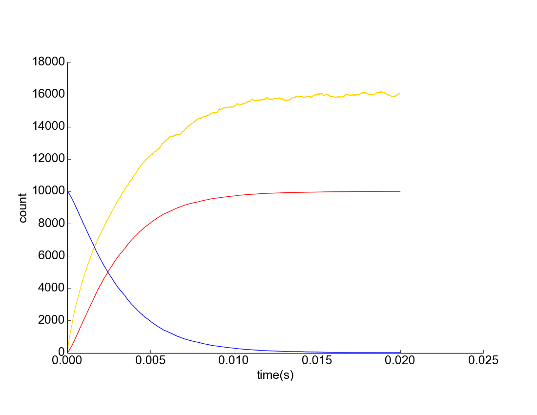
Figure 1. Upregulation of C. difficile Assuming Uniform Mixture. Yellow represents AIP concentration, Blue represents downregulated C. difficile population, Red represents upregulated C. difficile population.

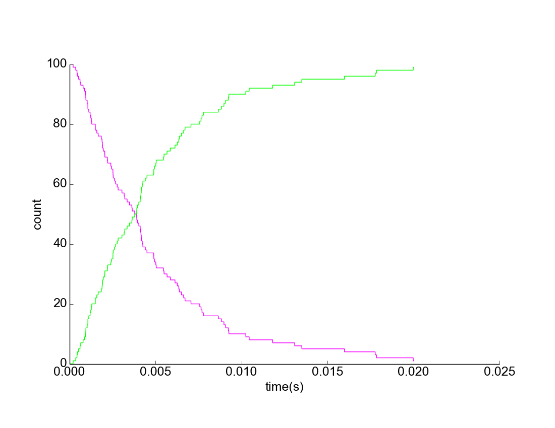
Figure 2. Upregulation of L. reuteri Assuming Uniform Mixture. Purple represents downregulated L. reuteri population; Green represents upregulated L. reuteri population.

As seen in Figures 1 and 2 above, assuming uniform mixture, upregulation of C. difficile and L. reuteri takes the same amount of time.

C. difficile and L. reuteri colonies assumed adjacent to each other.

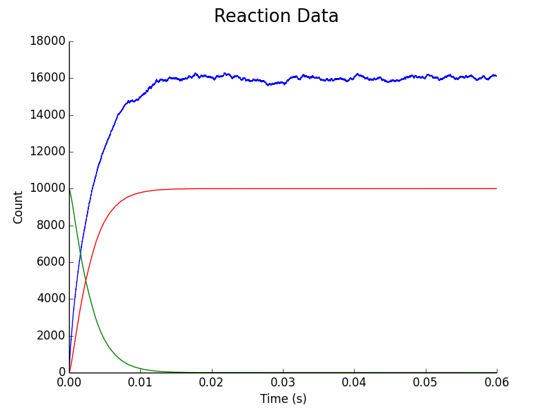
Figure 3. Upregulation of C. difficile assuming C. difficile & L. reuteri Colonies Adjacent. Blue represents AIP concentration, Green represents downregulated C. difficile population, Red represents upregulated C. difficile population.

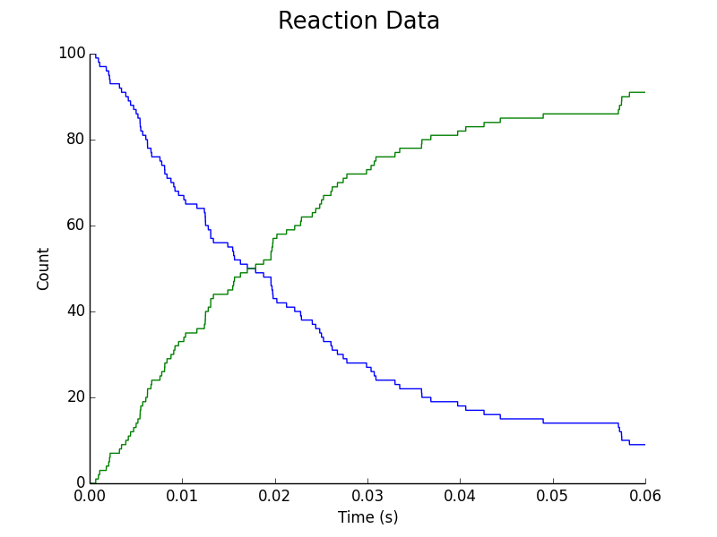
Figure 4. Upregulation of L. reuteri assuming C. difficile & L. reuteri Colonies Adjacent. Blue represents downregulated L. reuteri population; Green represents upregulated L. reuteri population.

In this case of the two bacterial colonies being spatially separated but adjacent, L. reuteri takes much longer to reach complete upregulation when compared to C. difficile. This is due to the greater diffusion distance of the AIP compared to in a uniform mixture.

C. difficile and L. reuteri colonies assumed spatially separated.

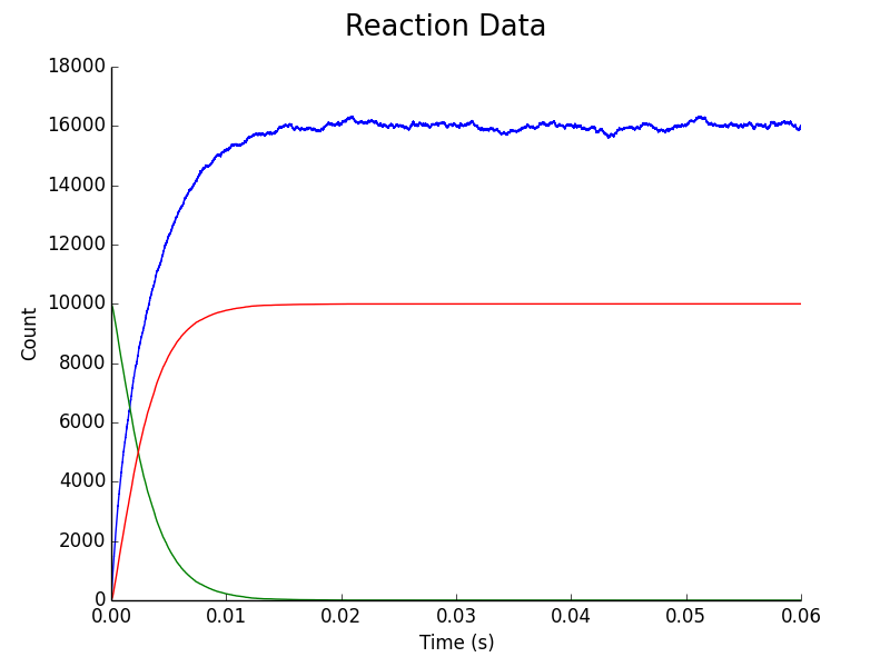
Figure 5. Upregulation of C. difficile assuming C. difficile & L. reuteri colonies are separated by a fixed distance in space. Blue represents AIP concentration; Green represents downregulated C. difficile population; Red represents upregulated C. difficile population.

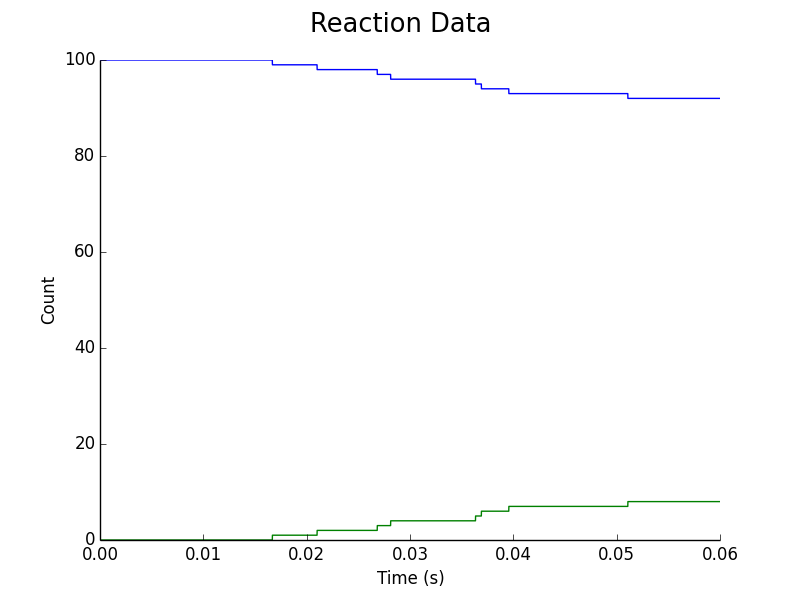
Figure 6. Upregulation of L. reuteri assuming C. difficile & L. reuteri colonies are separated by a fixed distance in space. Blue represents downregulated L. reuteri population, Green represents upregulated L. reuteri population.

Thus, as seen in Figure 6 above, spatial separation has resulted in a decrease in the upregulation of our probiotic to approximately 10%.

Discussion

We built a qualitative model to compare the upregulation of a C.difficile colony and a L. reuteri colony in different spatial orientations.

The results demonstrated that when both colonies were uniformly mixed, there is no significant delay in the upregulation of L. reuteri.

However, when both populations were placed adjacent to one another, only 50% of the L. reuteri upregulated in the time taken by C. difficile to upregulate. The percentage of upregulated cells decreased when a spatial separation was introduced. Such a spatial separation is equivalent to the distance diffused by the AIP molecule in the 0.06 second time range previously mentioned. In this case, only 10% of the probiotic’s population was upregulated.

It is evident that the relative spatial orientations of the bacteria makes a significant difference on the amount of AIP available to our probiotic. How can our system cope with the evident signal starvation?

A potential solution is a secondary amplification system that uses a separate signalling molecule in our system. Theoretically, it would mean that a small fraction of the L. reuteri being upregulated could trigger an upregulation cascade that triggers the production of endolysin in the rest of the population.

We analysed the suggested solution by adding another signal secretion & detection system, i.e., a secondary amplification system, into the models of our probiotic design.

Part II: Secondary Amplification System Spatial Model

Our first goal was to test whether a secondary amplification system would truly help to improve upregulation of our probiotic in different spatial orientations.

The following kinetic equations were then added to the previous spatial model:

Kinetic Equations & Kinetic Constants

Let the secondary amplification signalling molecule be denoted by S. For the secondary amplification system:

Kinetic Rate Equation	Kinetic Rate Constant	Kinetic Rate Constant Value Modelled
$$L. reuteri_{downregulated} \to L. reuteri_{downregulated} + S$$	$$k_S$$	$$10^{3} \ M \ s^{-1}$$
$$S \to [NULL]$$	$$\delta_S$$	$$10^{2} \ s^{-1}$$
$$L. reuteri_{downregulated} + S \to L. reuteri_{upregulated}$$	$$\gamma$$	$$10^{6} \ M^{-1} \ s^{-1}$$

Diffusion Constants

Species	Diffusion Rate Constant Value Modelled
$$AIP$$	$$10^{-9} \ cm^{2} \ s^{-1}$$

The kinetic rate constants of the secondary amplification signalling molecule were taken to be equivalent to that of AIP.

Results

On rerunning the simulation when the C. difficile and L. reuteri colonies are separated by a fixed distance in space, the following graph was obtained:

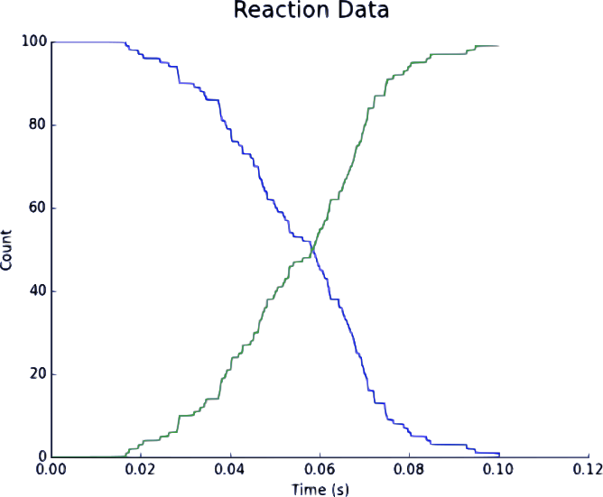
Figure 1. Upregulation of L. reuteriwith a Secondary Signalling System when C. difficile & L. reuteri are separated by a fixed distance in space. Blue represents downregulated L. reuteri population; Green represents upregulated L. reuteri population.

As seen in Figure 1 above, approximately 50% of the population is upregulated by time = 0.6 seconds. This is in contrast to the 10% upregulation obtained in the previous simulation without a secondary signalling system.

Discussion

Evidently, the implementation of a secondary amplification system into our model system has increased the upregulation of our probiotic in unfavourable spatial orientations.

After obtaining these results, we performed a quantitative mathematical analysis of the impact of a hypothetical secondary system on our probiotic’s response, the results of which are expanded on in the next part.

Part III: Secondary Signalling System Deterministic Model

To observe the efficacy of our engineered L. reuteri with a hypothetical secondary amplification system, we incorporated new differential equations into our existing deterministic mathematical model for the two-component regulatory system in the Model Design page and simulated this new integrated system.

Secondary Amplification System Primer

For our generic secondary amplification system, consider a signal X and its complementary receptor Y which can only be produced by previously AgrA/C-upregulated L. reuteri cells. The secreted signal X can then bind with the membrane receptor Y in neighbouring L. reuteri cells to form complex XY. This complex acts as a transcription factor that upregulates the L. reuteri cell.

Assumption

1. Signal X and receptor Y expression causes negligible cellular stress
2. Kinetic rates of the secondary amplification system are identical to those for the AgrAC two-component signalling system as in the Model Designpage.
3. Signal X and receptor Y can freely diffuse through cell membranes.
4. The upregulation profile due to signal-receptor complex XY can be approximated using an upregulation cut-off concentration as previously assumed for the AgrAC two-component signalling system.
5. A single molecule of signal-receptor complex XY is sufficient to cause upregulation. Consequently, the decrease in XY concentration can be ignored.

Kinetic Equations & Kinetic Rate Constants

Species Key

Transcription of Signalling Molecule X & Receptor Y

As previously described in the mathematical model for the AgrAC two-component signalling system, let the upregulation cut-off due to binding of dimerised phosphorylated AgrA be such that 10 pM of AIP can upregulated a single cell. This corresponds to a concentration of $$6.514 \times 10^{-9} \ M$$ of dimerised phosphorylated AgrA protein.

As mRNA transcription is triggered by dimerised, phosphorylated AgrA, the relevant kinetic equations are written as:

Kinetic Rate Equation	Kinetic Rate Constant	Kinetic Rate Constant Value Modelled
$$NULL \to M_{xy}$$	$$m_2 \ (if [Ap_2] \geq 6.514 \times 10^{-9} \ M); \\ 0 \ (if [Ap_2] \lt 6.514 \times 10^{-9} \ M)$$	$$8.33 \ M \ hour^{-1} \ cell^-1$$

Translation of Signalling Molecule & Receptor Y

Kinetic Rate Equation	Kinetic Rate Constant	Kinetic Rate Constant Value Modelled
$$M_{xy} \to X$$	$$v$$	$$1.67 \times 10^{-7} \ minutes^{-1}$$
$$M_{xy} \to Y$$	$$v$$	$$1.67 \times 10^{-7} \ minutes^{-1}$$

Ligand Binding of X to Receptor Y & Subsequent Formation of Transcription Factor

Kinetic Rate Equation	Kinetic Rate Constant	Kinetic Rate Constant Value Modelled
$$X + Y \to XY$$	$$k_{ir}$$	$$0.0167 \ M^{-1} \ minutes^{-1}$$

Upregulation of Cell by Transcription Factor of Secondary Signalling System

Kinetic Rate Constant	Kinetic Rate Constant Value Modelled
$$P$$	$$1 \ (if XY \geq 0.25 \times 10^{-5} \ M) \ or \ 0 \ (if XY \lt 0.25 \times 10^{-5} \ M)$$

Such a upregulation cutoff of XY was deliberately chosen so that small concentrations of XY transcription factor can upregulate the cell.

Degradation of Molecules

Kinetic Rate Equation	Kinetic Rate Constant	Kinetic Rate Constant Value Modelled
$$X \to NULL \ (where X=M_{xy}, X, Y)$$	$$\delta_X$$	$$0.0556 \ hour^{-1}$$

Differential Equations

Concentration Modelled	Differential Equation	Process Modelled
mRNA for Signaling Molecule X & Receptor Y	$$\frac {dM_{xy}}{dt} = m_2 - \delta_{M_{xy}} \times M_{xy}$$	Transcription + Degradation
Signalling Molecule X	$$\frac {dX}{dt} = v \times M_{xy} - k_{ir} \times X \times Y - \delta_X \times X$$	Translation + Ligand Binding + Degradation
Signalling Molecule Y	$$\frac {dY}{dt} = v \times M_{xy} - k_{ir} \times X \times Y - \delta_Y \times Y$$	Translation + Ligand Binding + Degradation
Ligand-Receptor Complex XY	$$\frac {dXY}{dt} = k_{ir} \times X \times Y - \delta_{XY} \times XY$$	Ligand Binding + Degradation

Results

To analyse the key features of the two-component regulatory system within each cell, we ran cellular-scale simulations in which the cell is exposed to various signal concentrations and patterns.

To see how the transcription factor changes during upregulation and downregulation, we input an AIP concentration of 1 nM at 350 hours, and removed it at 650 hours.

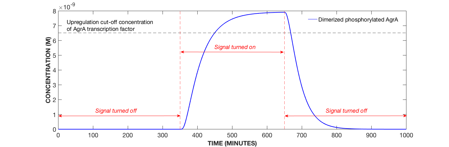
Figure 1. Dynamics of Dimerised, Phosphorylated AgrA Protein with Secondary Amplification System, AIP Concentration Modulated. Specifically, AIP added at 350 minutes and removed at 650 minutes.

The concentration of dimerized phosphorylated AgrA starts dropping immediately after the signal is taken away. It takes less than an hour to drop below the upregulation cut-off concentration.

\

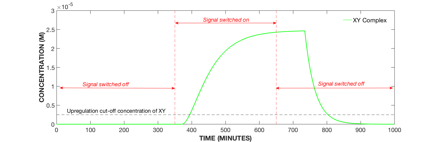
Figure 2. Dynamics of Signal-Receptor Complex XY with Secondary Amplification System, AIP Concentration Modulated. Specifically, AIP added at 350 minutes and removed at 650 minutes.

The concentration of the XY complex increases even after the signal has been switched off. This is because XY complex production is dependant on the upregulation of the cell, which in turn is controlled by the concentration by dimerized phosphorylated AgrA. As AgrA concentration takes some time to drop below it’s upregulation cut-off concentration, the XY complex is produced even after the signal is switched off.

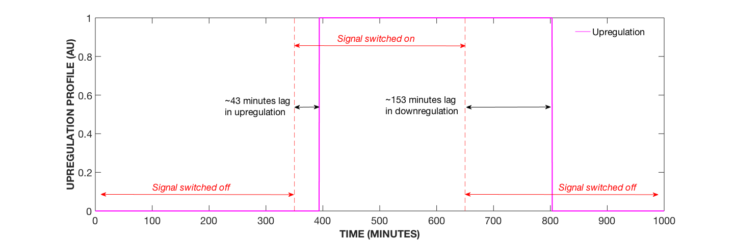
Figure 3. Upregulation Profile with Secondary Amplification System, AIP Concentration Modulated. Specifically, AIP added at 350 minutes and removed at 650 minutes.

The cell remains upregulated for a significant amount of time after the AIP signal switched off. The time lag is caused by:

1. Time taken by dimerized phosphorylated concentration to drop below its upregulation cut-off concentration.
2. Time taken by XY complex concentration to drop below its upregulation cut-off concentration.

Discussion

The graphs above depict the cell being upregulated for a considerable amount of time after dimerized phosphorylated AgrA has dropped below it’s cut-off upregulation concentration. This is caused by a cascade of delays in the response of the transcription factors to the loss of signal.

Therefore, not only does the secondary amplification system help trigger endolysin production in L. reuteri in unfavourable spatial orientations (as seen in previous sections), but it also maintains upregulation of the cell following signal depletion. This is beneficial for our probiotic as it increases therapeutic efficacy in its suppression of C. difficile pathogenicity.

References

Reference
Stiles, JR, et al. (1996). Miniature endplate current rise times < 100 μs from improved dual recordings can be modeled with passive acetylcholine diffusion from a synaptic vesicle. Proc. Natl. Acad. Sci. USA 93:5747-5752.
Jabbari, Sara, et al. “Mathematical Modelling of the Agr Operon in Staphylococcus Aureus.” Journal of Mathematical Biology, vol. 61, no. 1, 2009, pp. 17–54., doi:10.1007/s00285-009-0291-6.
Stiles, JR, and Bartol, TM. (2001). Monte Carlo methods for simulating realistic synaptic microphysiology using MCell. In: Computational Neuroscience: Realistic Modeling for Experimentalists, ed. De Schutter, E. CRC Press, Boca Raton, pp. 87-127.
Kerr R, Bartol TM, Kaminsky B, Dittrich M, Chang JCJ, Baden S, Sejnowski TJ, Stiles JR. (2009). Fast Monte Carlo Simulation Methods for Biological Reaction-Diffusion Systems in Solution and on Surfaces. SIAM J. Sci. Comput., 30(6):3126-3149.